
Market Microstructure in MQL5 (Part 4): Volatility That Remembers

Introduction
Part 1 built a defensive foundation: guarded math, validated price feeds, and stable statistical primitives. Part 2 added confidence-weighted Hurst estimation, establishing that US100 M1 Globex operates near the random-walk boundary (pooled H = 0.511, rolling H ≈ 0.48). Part 3 added the GPH estimator for the fractional differencing parameter d, with pooled d = −0.006 and session-to-session standard deviation of 0.153.
Standard volatility indicators — ATR and standard deviation of returns — treat each bar as independent. They ignore four empirical facts about financial volatility: clustering (large moves follow large moves), persistence (volatility shocks decay slowly), asymmetry (negative returns increase future volatility more than positive returns of the same magnitude), and regime mixing (the series may be a mixture of different scaling laws, making average measures like H and d misleading). On intraday US100 M1 data, these properties directly affect position sizing, stop-loss placement, and signal filtering. A trading system that ignores them is systematically miscalibrated.
This article adds two measurement families to MicroStructure_Foundation.mqh: (1) a revised MFDFA-based multifractal spectrum that returns Δα with an R² confidence field, replacing the raw τ-spread proxy used in the original submission; (2) a volatility suite: RealizedVolatility(), DurationVolatility(), FractionalVolatility(), a FIGARCH-inspired proxy, VolatilityClusteringIndex(), LeverageEffect(), JumpIntensity(), and PopulateVolatilityAnalysis().
The empirical study in this article uses NQ E-mini Nasdaq 100 futures (CME Globex) rather than the US100 CFD instrument referenced in earlier drafts. NQ is the exchange-traded underlying contract; US100 is a retail CFD product whose price is derived from the index, not from actual futures order flow. The microstructure properties being measured — volatility clustering, leverage asymmetry, jump intensity, multifractal structure — are properties of price formation at the exchange level. Using the actual futures contract is therefore a more appropriate methodological choice for this analysis. The 2-year NQ M1 dataset (514 NY sessions, May 2024–May 2026) captures four macro stress episodes relevant to this series: the BoJ carry-trade unwind of August 2024, the Fed hawkish surprise of December 2024, the Liberation Day tariff shock of April 2025, and the second tariff episode of April 2026.
Before the implementation sections, several points require explicit framing.
FIGARCHVolatility() is not a fitted FIGARCH model. A proper FIGARCH estimation requires maximum-likelihood optimization over hundreds of observations and is computationally unsuitable for real-time MQL5 use. The function implemented here is a power-law weighted realized volatility, where the weights are derived from the GPH d estimate produced by Part 3. It is a FIGARCH-inspired engineering proxy. It captures the memory structure of the volatility process without the estimation overhead of a full FIGARCH specification.
LeverageEffect() uses a fitted GJR-GARCH(1,1,1) model via the Dube volatility library (Yun, 2026). This is a genuine model estimation, not a heuristic. It returns the normalized asymmetry ratio γ/(α + γ + β), which is scale-independent and directly comparable across sessions. A compile-time flag controls whether the Dube library path or a simpler fallback is used; both paths are described in the folder structure section.
JumpIntensity() uses bipower variation as the threshold baseline. This is more robust than a simple σ-threshold, but it is still a relative flag rather than a formal jump test.
Deliverable: eight functions updated or added to MicroStructure_Foundation.mqh, a revised MFDFA returning Δα with R² confidence, and the VolatilityAnalysis struct fully populated with no placeholder fields. No new include file is created. The two companion SSRN working papers that document the empirical foundation for this series are available at SSRN 6809080 and SSRN 6847024.
The Stylized Facts of Volatility
Volatility clustering means that large price changes tend to be followed by large price changes (of either sign), and small changes by small changes. Engle (1982) formalized this as the ARCH effect, for which he received the Nobel Prize. The lag-1 autocorrelation of squared returns is a direct measure of clustering. Values above 0.2 on daily data are typical; on intraday data, clustering is often stronger. VolatilityClusteringIndex() measures this directly. It is a diagnostic proxy, not a fitted model.
Volatility persistence means that shocks to volatility decay slowly — not exponentially as GARCH(1,1) implies, but hyperbolically. The fractional differencing parameter d from Part 3 quantifies this: when d > 0 for the squared-return series, volatility itself has long memory. FractionalVolatility() uses that d directly, connecting this article to Part 3 by design. The key simplification is that d is estimated from the return series and applied to squared returns. This assumes the same memory parameter for returns and volatility. It is a reasonable approximation for intraday equity data but is not guaranteed.
The leverage effect (Black, 1976) describes the asymmetric response: negative returns increase future volatility more than positive returns of the same magnitude. The standard model for this effect is GJR-GARCH (Glosten, Jagannathan and Runkle, 1993), which adds a single asymmetry parameter γ to the GARCH(1,1) specification: σ² t = ω + α·ε² t−1 + γ·I t−1 ·ε² t−1 + β·σ² t−1 , where I t−1 = 1 if the previous return was negative. LeverageEffect() fits this model via the Dube library and returns the normalized ratio γ/(α + γ + β).
Volatility jumps are rare but consequential. Andersen, Bollerslev and Diebold (2007) proposed bipower variation (BPV = (π/2)·mean(|r t |·|r t−1 |)) as a jump-robust baseline. JumpIntensity() uses BPV as the threshold rather than the sample standard deviation, because a simple σ-threshold is contaminated by the very jumps it is trying to detect. On NQ M1, the 514-session empirical study shows a mean jump intensity of 1.4% with a 90th percentile of 2.1%. A value above 5% is likely to indicate data artifacts — bad ticks, contract rollovers, or feed anomalies — rather than genuine market jumps.
Multifractality measures whether the series follows a single scaling law or a mixture. The conventional width metric is Δα = α max − α min , where α(q) is the Hölder exponent obtained via the Legendre transform of τ(q) = q·h(q) − 1. The revised MultifractalSpectrum() computes this properly and stores the mean R² of the scaling regressions as a confidence field. A narrow Δα (< 0.3) means H and d are reliable descriptors. A wide Δα (> 0.5) means the series contains opposing memory regimes that cancel in the average.
Implementation 1: Revised Multifractal Spectrum (MFDFA)
The MFDFA algorithm is unchanged in structure. The revision affects the output metric only: the raw τ-spread is replaced by the Legendre-transform Δα, and the function now accepts a confidence output parameter. The outlier filter (|r| ≥ 0.1) is retained; it removes contract rollovers and bad ticks that would otherwise distort the negative-q moments, where large fluctuations dominate the q-th power sum.
The Legendre transform proceeds as follows. From each q-regression, the slope h(q) is stored. The Hölder exponent is α(q) = h(q) + q·h′(q), where h′(q) is approximated by central finite differences. The spectrum width is Δα = max(α) − min(α). The confidence is the mean R² across all q-regressions; a value below 0.65 indicates unreliable scaling and the result should be treated as unavailable.
//+------------------------------------------------------------------+
//| MultifractalSpectrum: MFDFA returning Legendre-transform Δα.     |
//| confidence = mean R² of the log(F) ~ log(s) regressions.         |
//| Returns Δα = max(α) − min(α). Returns 0.0 on failure.            |
//|                                                                  |
//| Outlier filter: |r| >= 0.1 removed before profile construction.  |
//| MFDFA is sensitive to extreme values at negative q because large |
//| fluctuations dominate the q-th moment. Rollovers and bad ticks   |
//| must be excluded before the profile is built.                    |
//+------------------------------------------------------------------+
double MultifractalSpectrum(const string symbol, const int tf,
                             const int period, double &confidence,
                             int q_min = -5, int q_max = 5)
  {
   confidence = 0.0;
   if(!ValidateSymbolV2(symbol) || period < 100)
      return 0.0;
   double close[];
   if(SafeCopyClose(symbol, tf, 0, period + 1, close) < period + 1)
      return 0.0;
   //--- Build log-return array; filter gross outliers
   double returns[];
   ArrayResize(returns, period);
   int valid = 0;
   for(int i = 0; i < period; i++)
     {
      if(close[i] <= 0.0 || close[i + 1] <= 0.0) continue;
      double r = SafeLog(close[i + 1]) - SafeLog(close[i]);
      if(MathAbs(r) < 0.1) returns[valid++] = r;
     }
   if(valid < 100) return 0.0;
   ArrayResize(returns, valid);
   //--- Cumulative sum profile (demeaned)
   double mean_r = 0.0;
   for(int i = 0; i < valid; i++) mean_r += returns[i];
   mean_r /= valid;
   double y[];
   ArrayResize(y, valid);
   double cum = 0.0;
   for(int i = 0; i < valid; i++) { cum += returns[i] - mean_r; y[i] = cum; }
   //--- Geometric scales (powers of two); minimum 4 full segments.
   //--- Minimum scale = 16: below this, linear detrending is unreliable
   //--- on noisy M1 data. Maximum = valid/4 ensures 4 full segments.
   int scales[];
   int max_scale = valid / 4, s = 16, scale_count = 0;
   while(s <= max_scale)
     { ArrayResize(scales, scale_count + 1); scales[scale_count++] = s; s *= 2; }
   if(scale_count < 2) return 0.0;
   //--- q values
   int    q_cnt = q_max - q_min + 1;
   double q_vals[], h_q[];
   ArrayResize(q_vals, q_cnt);
   ArrayResize(h_q,   q_cnt);
   ArrayInitialize(h_q, 0.0);
   for(int qi = 0; qi < q_cnt; qi++) q_vals[qi] = q_min + qi;
   double r2_sum = 0.0;
   int    r2_cnt = 0;
   for(int qi = 0; qi < q_cnt; qi++)
     {
      double q = q_vals[qi];
      double logF[], logS[];
      int points = 0;
      for(int sidx = 0; sidx < scale_count; sidx++)
        {
         int seg_s = scales[sidx], n_seg = valid / seg_s;
         if(n_seg < 2) continue;
         double F_sum = 0.0;
         int    seg_cnt = 0;
         for(int v = 0; v < n_seg; v++)
           {
            int    start = v * seg_s;
            double sx = 0.0, sy = 0.0, sxy = 0.0, sxx = 0.0;
            for(int k = 0; k < seg_s; k++)
              { sx += k; sy += y[start+k]; sxy += k*y[start+k]; sxx += k*k; }
            double dn = seg_s * sxx - sx * sx;
            if(MathAbs(dn) < DBL_MIN_POSITIVE) continue;
            double sl = (seg_s*sxy - sx*sy)/dn, ic = (sy - sl*sx)/seg_s;
            double var = 0.0;
            for(int k = 0; k < seg_s; k++)
              { double res = y[start+k] - (ic + sl*k); var += res*res; }
            var /= seg_s;
            if(q == 0.0) F_sum += MathLog(MathMax(var, DBL_MIN_POSITIVE));
            else         F_sum += MathPow(MathMax(var, DBL_MIN_POSITIVE), q/2.0);
            seg_cnt++;
           }
         if(seg_cnt == 0) continue;
         double Fq = (q == 0.0) ? MathExp(F_sum/seg_cnt)
                                 : MathPow(F_sum/seg_cnt, 1.0/q);
         if(Fq <= DBL_MIN_POSITIVE) continue;
         ArrayResize(logF, points+1); ArrayResize(logS, points+1);
         logF[points] = MathLog(Fq); logS[points] = MathLog((double)seg_s);
         points++;
        }
      if(points < 2) continue;
      double lsx=0,lsy=0,lsxy=0,lsxx=0;
      for(int p=0;p<points;p++){lsx+=logS[p];lsy+=logF[p];lsxy+=logS[p]*logF[p];lsxx+=logS[p]*logS[p];}
      double den = points*lsxx - lsx*lsx;
      if(MathAbs(den) < DBL_MIN_POSITIVE) continue;
      h_q[qi] = (points*lsxy - lsx*lsy) / den;
      //--- R² for this q regression
      double ym=lsy/points, ss_tot=0, ss_res=0;
      double pi_int = (lsy - h_q[qi]*lsx)/points;
      for(int p=0;p<points;p++)
        {
         double pr = pi_int + h_q[qi]*logS[p];
         ss_res += (logF[p]-pr)*(logF[p]-pr);
         ss_tot += (logF[p]-ym)*(logF[p]-ym);
        }
      if(ss_tot > DBL_MIN_POSITIVE) { r2_sum += 1.0 - ss_res/ss_tot; r2_cnt++; }
     }
   if(r2_cnt > 0) confidence = r2_sum / r2_cnt;
   //--- Legendre transform: α(q) = h(q) + q·h'(q)
   //--- h'(q) by central finite differences
   double alpha[];
   ArrayResize(alpha, q_cnt);
   for(int qi = 0; qi < q_cnt; qi++)
     {
      double dh;
      if(qi == 0)          dh = h_q[1] - h_q[0];
      else if(qi == q_cnt-1) dh = h_q[q_cnt-1] - h_q[q_cnt-2];
      else                  dh = (h_q[qi+1] - h_q[qi-1]) / 2.0;
      alpha[qi] = h_q[qi] + q_vals[qi] * dh;
     }
   double amax = alpha[0], amin = alpha[0];
   for(int qi = 1; qi < q_cnt; qi++)
     { if(alpha[qi] > amax) amax=alpha[qi]; if(alpha[qi] < amin) amin=alpha[qi]; }
   double delta_alpha = amax - amin;
   if(!MathIsValidNumber(delta_alpha) || delta_alpha > 10.0) return 0.0;
   return MathMax(0.0, delta_alpha);
  }

//+------------------------------------------------------------------+
//| PopulateMultifractalAnalysis: writes multifractal_width (Δα) and |
//| dimension_confidence (mean R²) into RobustFractalAnalysis.       |
//| Sessions with confidence < 0.65 have unreliable Δα estimates.    |
//+------------------------------------------------------------------+
void PopulateMultifractalAnalysis(const string symbol, const int tf,
                                   const int period, RobustFractalAnalysis &result)
  {
   result.multifractal_width    = 0.0;
   result.dimension_confidence  = 0.0;
   if(!ValidateSymbolV2(symbol) || period < 100) return;
   double conf = 0.0;
   double width = MultifractalSpectrum(symbol, tf, period, conf);
   if(MathIsValidNumber(width))       result.multifractal_width   = width;
   if(MathIsValidNumber(conf))        result.dimension_confidence = conf;
  }
Implementation 2: Realized and Duration-Adjusted Volatility
RealizedVolatility() returns the square root of the mean of squared log-returns. It is the benchmark estimator: it makes no assumption about memory or regime structure. DurationVolatility() annualizes RV using the bar duration. The original implementation used 252 × 86,400 seconds as the denominator, which assumes round-the-clock trading. The NY session runs 09:30–16:00 ET — 23,400 seconds per day. The corrected function uses 23,400 for M1 data and the full-day figure for daily and higher timeframes.
//+------------------------------------------------------------------+
//| RealizedVolatility: sqrt(mean(squared log-returns))              |
//+------------------------------------------------------------------+
double RealizedVolatility(const string symbol, const int tf,
                           const int window, int shift = 0)
  {
   if(!ValidateSymbolV2(symbol) || window < 2) return 0.0;
   double close[];
   if(SafeCopyClose(symbol, tf, shift, window + 1, close) < window + 1) return 0.0;
   int    n_returns = ArraySize(close) - 1;
   double sum_sq = 0.0;
   int    valid  = 0;
   for(int i = 0; i < n_returns; i++)
     {
      if(close[i] <= 0.0 || close[i+1] <= 0.0) continue;
      double r = SafeLog(close[i+1]) - SafeLog(close[i]);
      sum_sq += r * r; valid++;
     }
   if(valid == 0) return 0.0;
   return MathSqrt(sum_sq / valid);
  }

//+------------------------------------------------------------------+
//| DurationVolatility: session-aware annualized realized volatility.|
//| Uses NY session seconds (23,400) for M1; full-day (86,400) for   |
//| H1 and above. The previous version used 86,400 for all frames,   |
//| which overstated annualized vol for session-filtered M1 data.    |
//+------------------------------------------------------------------+
double DurationVolatility(const string symbol, const int tf,
                           const int bars, int shift = 0)
  {
   if(!ValidateSymbolV2(symbol) || bars < 2) return 0.0;
   double close[];
   if(SafeCopyClose(symbol, tf, shift, bars + 1, close) < bars + 1) return 0.0;
   int    n_returns = ArraySize(close) - 1;
   double sum_sq = 0.0;
   int    valid  = 0;
   for(int i = 0; i < n_returns; i++)
     {
      if(close[i] <= 0.0 || close[i+1] <= 0.0) continue;
      double r = SafeLog(close[i+1]) - SafeLog(close[i]);
      sum_sq += r * r; valid++;
     }
   if(valid == 0) return 0.0;
   double realized = MathSqrt(sum_sq / valid);
   int    tf_sec   = PeriodSeconds(tf);
   if(tf_sec <= 0) return 0.0;
   //--- NY session = 23,400 s for M1; full day for longer frames
   double day_sec    = (tf == PERIOD_M1) ? 23400.0 : 86400.0;
   double ann_factor = MathSqrt(252.0 * day_sec / tf_sec);
   return realized * ann_factor;
  }
Implementation 3: Fractional Volatility
FractionalVolatility() applies the ARFIMA memory kernel to squared returns. Weights decay as kd−1, where k is the lag and d is the GPH estimate from Part 3. When d = 0, the weights are flat and the result equals standard realized volatility. When d > 0, distant observations receive relatively more weight; the volatility estimate incorporates long-range structure. When d < 0, weights decay faster than a uniform average, reflecting anti-persistence.
//+------------------------------------------------------------------+
//| FractionalVolatility: ARFIMA memory-kernel weighted volatility.  |
//| Weights: w_k = k^(d-1). When d = 0, equals realized volatility.  |
//| Simplification: d from returns applied to squared returns.       |
//| This assumes return memory and volatility memory share the same  |
//| parameter — reasonable for intraday equity, not guaranteed.      |
//+------------------------------------------------------------------+
double FractionalVolatility(const string symbol, const int tf,
                             const int window, double d = -1.0)
  {
   if(!ValidateSymbolV2(symbol) || window < 5) return 0.0;
   double close[];
   if(SafeCopyClose(symbol, tf, 0, window + 1, close) < window + 1) return 0.0;
   int n_returns = ArraySize(close) - 1;
   if(n_returns < 4) return 0.0;
   double returns[];
   ArrayResize(returns, n_returns);
   int valid_ret = 0;
   for(int i = 0; i < n_returns; i++)
     {
      if(close[i] <= 0.0 || close[i+1] <= 0.0) continue;
      double r = SafeLog(close[i+1]) - SafeLog(close[i]);
      if(MathAbs(r) < 0.1) returns[valid_ret++] = r;
     }
   if(valid_ret < 5) return 0.0;
   ArrayResize(returns, valid_ret);
   if(d <= -0.49 || d >= 0.49)
     { double conf_dummy; d = GPHEstimator(returns, valid_ret, conf_dummy); }
   d = MathMax(-0.49, MathMin(0.49, d));
   double sum_w = 0.0, sum_wrr = 0.0;
   for(int k = 1; k <= valid_ret; k++)
     {
      double w = MathPow((double)k, d - 1.0);
      if(!MathIsValidNumber(w) || w > 1e10) w = 1.0;
      sum_w   += w;
      sum_wrr += w * returns[valid_ret - k] * returns[valid_ret - k];
     }
   if(sum_w <= DBL_MIN_POSITIVE) return 0.0;
   return MathSqrt(MathMax(0.0, sum_wrr / sum_w));
  }
Implementation 4: FIGARCH-Inspired Proxy
FIGARCHVolatility() is not a fitted FIGARCH model. A full FIGARCH requires maximum-likelihood estimation, which is computationally unsuitable for real-time M1 use on sessions of 390 bars. The function is a power-law weighted conditional variance proxy, where the weight recursion w j = w j−1 ·(j−1−d)/j is the truncated fractional differencing kernel of Baillie et al. (1996), applied directly to squared returns. The baseline variance uses bipower variation rather than the sample mean, making the floor robust to isolated jump returns. The original hardcoded omega = 1e-6 and beta = 0.85 are removed; the function now relies entirely on the GPH d from Part 3 and the bipower baseline.
//+------------------------------------------------------------------+
//| FIGARCHVolatility: FIGARCH-inspired power-law conditional proxy. |
//|                                                                  |
//| THIS IS NOT A FITTED FIGARCH MODEL. It is a power-law weighted   |
//| realized volatility proxy using the fractional differencing      |
//| kernel of Baillie et al. (1996). The memory exponent d comes     |
//| from the Part 3 GPH estimate. The baseline is bipower variation, |
//| which is robust to isolated jump returns.                        |
//+------------------------------------------------------------------+
double FIGARCHVolatility(const string symbol, const int tf,
                          const int window, double d = -1.0)
  {
   if(!ValidateSymbolV2(symbol) || window < 20) return 0.0;
   double close[];
   if(SafeCopyClose(symbol, tf, 0, window + 2, close) < window + 2) return 0.0;
   int n_returns = ArraySize(close) - 1;
   if(n_returns < 20) return 0.0;
   double returns[];
   ArrayResize(returns, n_returns);
   int valid_ret = 0;
   for(int i = 0; i < n_returns; i++)
     {
      if(close[i] <= 0.0 || close[i+1] <= 0.0) continue;
      double r = SafeLog(close[i+1]) - SafeLog(close[i]);
      if(MathAbs(r) < 0.1) returns[valid_ret++] = r;
     }
   if(valid_ret < 20) return 0.0;
   ArrayResize(returns, valid_ret);
   if(d <= -0.49 || d >= 0.49)
     { double conf_dummy; d = GPHEstimator(returns, valid_ret, conf_dummy); }
   d = MathMax(-0.49, MathMin(0.49, d));
   //--- Bipower variation baseline: BPV = (π/2)·mean(|r_t|·|r_{t-1}|)
   //--- Robust to isolated jumps: a single large return contaminates
   //--- at most two adjacent products, leaving the mean stable.
   double bpv_sum = 0.0;
   int    bpv_cnt = 0;
   for(int i = 1; i < valid_ret; i++)
     { bpv_sum += MathAbs(returns[i]) * MathAbs(returns[i-1]); bpv_cnt++; }
   double baseline_var = (bpv_cnt > 0)
                         ? (M_PI/2.0) * bpv_sum / bpv_cnt : 0.0;
   //--- Fractional differencing kernel: w_0 = 1; w_j = w_{j-1}*(j-1-d)/j
   int    L = MathMin(100, valid_ret - 1);
   double weights[];
   ArrayResize(weights, L);
   weights[0] = 1.0;
   for(int j = 1; j < L; j++)
     {
      weights[j] = weights[j-1] * (j - 1.0 - d) / (double)j;
      if(!MathIsValidNumber(weights[j]) || MathAbs(weights[j]) > 1e6)
         weights[j] = 0.0;
     }
   double cond_var = 0.0, sum_w = 0.0;
   for(int j = 0; j < L; j++)
     {
      int idx = valid_ret - 1 - j;
      if(idx < 0) break;
      cond_var += weights[j] * returns[idx] * returns[idx];
      sum_w    += weights[j];
     }
   if(sum_w > DBL_MIN_POSITIVE) cond_var /= sum_w;
   else                          cond_var  = baseline_var;
   cond_var = MathMax(cond_var, baseline_var);
   if(cond_var <= 0.0) return 0.0;
   return MathSqrt(cond_var);
  }
Implementation 5: Clustering Index, GJR Leverage Effect, Bipower Jump Intensity
VolatilityClusteringIndex() is unchanged: it returns the lag-1 autocorrelation of squared returns, which is a direct diagnostic for the ARCH effect.
LeverageEffect() is substantially revised. The original implementation measured the ratio of next-bar variance after negative versus positive returns — a simple heuristic, not a recognized leverage effect model. The revision fits a GJR-GARCH(1,1,1) model via the Dube volatility library and returns the normalized asymmetry ratio γ/(α + γ + β). This ratio is scale-independent, stationary-constrained (the function returns 0.0 if α + γ/2 + β ≥ 1), and directly comparable across sessions. A compile-time flag USE_GJR_LEVERAGE controls the path. If the Dube library is not installed, the function compiles and runs using the original sign-conditioned variance fallback.
JumpIntensity() now uses bipower variation as the baseline rather than the sample standard deviation. A return is classified as a jump when its squared value exceeds σ mult ² × BPV. This is more robust because the sample σ is inflated by the very returns it is trying to classify.
//+------------------------------------------------------------------+
//| VolatilityClusteringIndex: lag-1 autocorrelation of squared rets |
//| Diagnostic for the ARCH effect. Values above 0.1 confirm         |
//| clustering; above 0.2 indicate strong, predictable volatility.   |
//+------------------------------------------------------------------+
double VolatilityClusteringIndex(const string symbol, const int tf,
                                   const int window)
  {
   if(!ValidateSymbolV2(symbol) || window < 3) return 0.0;
   double close[];
   if(SafeCopyClose(symbol, tf, 0, window + 1, close) < window + 1) return 0.0;
   int    n_returns = ArraySize(close) - 1;
   if(n_returns < 3) return 0.0;
   double sq_ret[];
   ArrayResize(sq_ret, n_returns);
   int    valid = 0;
   for(int i = 0; i < n_returns; i++)
     {
      if(close[i] <= 0.0 || close[i+1] <= 0.0) continue;
      double r = SafeLog(close[i+1]) - SafeLog(close[i]);
      sq_ret[valid++] = r * r;
     }
   if(valid < 3) return 0.0;
   ArrayResize(sq_ret, valid);
   double mean = 0.0;
   for(int i = 0; i < valid; i++) mean += sq_ret[i];
   mean /= valid;
   double num = 0.0, den = 0.0;
   for(int i = 0; i < valid - 1; i++)
     {
      num += (sq_ret[i] - mean) * (sq_ret[i+1] - mean);
      den += (sq_ret[i] - mean) * (sq_ret[i]   - mean);
     }
   if(den <= DBL_MIN_POSITIVE) return 0.0;
   return MathMax(-1.0, MathMin(1.0, num / den));
  }

//+------------------------------------------------------------------+
//| LeverageEffect: GJR-GARCH(1,1,1) asymmetry parameter.            |
//| Returns γ/(α + γ + β) in [0, 1] — normalized, scale-free.        |
//|                                                                  |
//| Requires Dube volatility library. Add before your #include:      |
//|   #define USE_GJR_LEVERAGE                                       |
//| Without this define, falls back to next-bar variance asymmetry.  |
//| Returns 0.0 if model fails to converge or stationarity           |
//| condition α + γ/2 + β >= 1 is violated.                          |
//+------------------------------------------------------------------+
double LeverageEffect(const string symbol, const int tf,
                        const int window)
  {
   if(!ValidateSymbolV2(symbol) || window < 30) return 0.0;
   double close[];
   if(SafeCopyClose(symbol, tf, 0, window + 1, close) < window + 1) return 0.0;
   int    n_returns = ArraySize(close) - 1;
   if(n_returns < 30) return 0.0;
   double SCALE = 100.0;
   double returns[];
   ArrayResize(returns, n_returns);
   int    valid = 0;
   for(int i = 0; i < n_returns; i++)
     {
      if(close[i] <= 0.0 || close[i+1] <= 0.0) continue;
      double r = SafeLog(close[i+1]) - SafeLog(close[i]);
      if(MathAbs(r) < 0.1) returns[valid++] = r * SCALE;
     }
   if(valid < 30) return 0.0;
   ArrayResize(returns, valid);

#ifdef USE_GJR_LEVERAGE
   //--- GJR-GARCH path (Dube library required)
   //--- Model: σ²_t = ω + α·ε²_{t-1} + γ·I_{t-1}·ε²_{t-1} + β·σ²_{t-1}
   //--- params order after fit(): [mu, omega, alpha, gamma, beta]
   vector obs;
   obs.Init(valid);
   for(int i = 0; i < valid; i++) obs[i] = returns[i];
   ArchParameters spec;
   spec.observations     = obs;
   spec.include_constant = true;
   spec.vol_model_type   = VOL_GJR_GARCH;
   spec.garch_p = 1;
   spec.garch_o = 1;
   spec.garch_q = 1;
   ConstantMean gjr_model;
   if(!gjr_model.initialize(spec)) return 0.0;
   ArchModelResult res = gjr_model.fit(SCALE);
   if(!res.params.Size()) return 0.0;
   double alpha = res.params[2];
   double gamma = res.params[3];
   double beta  = res.params[4];
   if((alpha + gamma/2.0 + beta) >= 1.0) return 0.0;  // stationarity
   if(alpha < 0.0 || gamma < 0.0 || beta < 0.0)  return 0.0;
   double denom = alpha + gamma + beta;
   if(denom <= DBL_MIN_POSITIVE) return 0.0;
   return MathMax(0.0, MathMin(1.0, gamma / denom));
#else
   //--- Fallback: next-bar variance asymmetry proxy
   //--- Measures sign-conditioned next-bar squared return ratio.
   //--- Less rigorous than GJR-GARCH; requires no external library.
   double sum_sq_neg = 0.0, sum_sq_pos = 0.0;
   int    cnt_neg = 0, cnt_pos = 0;
   for(int i = 0; i < valid - 1; i++)
     {
      double v = returns[i+1] * returns[i+1];
      if(returns[i] < 0.0) { sum_sq_neg += v; cnt_neg++; }
      else                  { sum_sq_pos += v; cnt_pos++; }
     }
   if(cnt_neg == 0 || cnt_pos == 0) return 0.0;
   double vn = sum_sq_neg/cnt_neg, vp = sum_sq_pos/cnt_pos;
   double dn = vn + vp;
   if(dn <= DBL_MIN_POSITIVE) return 0.0;
   return MathMax(-1.0, MathMin(1.0, (vn - vp) / dn));
#endif
  }

//+------------------------------------------------------------------+
//| JumpIntensity: proportion of returns classified as jumps.        |
//| Baseline: bipower variation BPV = (π/2)·mean(|r_t|·|r_{t-1}|).   |
//| A return is a jump when r²_t > sigma_mult² × BPV.                |
//| BPV is robust to isolated jumps; sample σ is not.                |
//| Values above 2% indicate elevated activity; above 5% indicates   |
//| data artifacts (bad ticks, rollovers). Reject if > 5%.           |
//+------------------------------------------------------------------+
double JumpIntensity(const string symbol, const int tf,
                      const int window, double sigma_mult = 3.0)
  {
   if(!ValidateSymbolV2(symbol) || window < 5 || sigma_mult <= 0.0) return 0.0;
   double close[];
   if(SafeCopyClose(symbol, tf, 0, window + 1, close) < window + 1) return 0.0;
   int    n_returns = ArraySize(close) - 1;
   if(n_returns < 5) return 0.0;
   double returns[];
   ArrayResize(returns, n_returns);
   int    valid = 0;
   for(int i = 0; i < n_returns; i++)
     {
      if(close[i] <= 0.0 || close[i+1] <= 0.0) continue;
      double r = SafeLog(close[i+1]) - SafeLog(close[i]);
      if(MathIsValidNumber(r)) returns[valid++] = r;
     }
   if(valid < 5) return 0.0;
   ArrayResize(returns, valid);
   //--- Bipower variation baseline
   double bpv_sum = 0.0;
   for(int i = 1; i < valid; i++)
      bpv_sum += MathAbs(returns[i]) * MathAbs(returns[i-1]);
   double bpv = (valid > 1) ? (M_PI/2.0) * bpv_sum / (valid - 1) : 0.0;
   if(bpv <= DBL_MIN_POSITIVE) return 0.0;
   double threshold_sq = sigma_mult * sigma_mult * bpv;
   int    jumps = 0;
   for(int i = 0; i < valid; i++)
      if(returns[i] * returns[i] > threshold_sq) jumps++;
   return (double)jumps / valid;
  }
Implementation 6: PopulateVolatilityAnalysis Wrapper
The wrapper signature is unchanged from the original submission. The asymmetry field is now populated with the standardized skewness of log-returns — a distributional diagnostic — rather than a hardcoded zero. The volatility_confidence field in RobustFractalAnalysis is set to the clustering index as before.
//+------------------------------------------------------------------+
//| PopulateVolatilityAnalysis: fills all VolatilityAnalysis fields. |
//| asymmetry = standardized skewness of log-returns.                |
//| This is a distributional diagnostic. The volatility asymmetry    |
//| is captured separately by leverage_effect (GJR γ ratio).         |
//+------------------------------------------------------------------+
void PopulateVolatilityAnalysis(const string symbol, const int tf,
                                  const int period, VolatilityAnalysis &result,
                                  RobustFractalAnalysis &rfa)
  {
   result.realized_vol     = RealizedVolatility(symbol, tf, period, 0);
   result.duration_vol     = DurationVolatility(symbol, tf, period, 0);
   result.fractional_vol   = FractionalVolatility(symbol, tf, period, -1.0);
   result.figarch_vol      = FIGARCHVolatility(symbol, tf, period, -1.0);
   result.clustering_index = VolatilityClusteringIndex(symbol, tf, period);
   result.leverage_effect  = LeverageEffect(symbol, tf, period);
   result.jump_intensity   = JumpIntensity(symbol, tf, period, 3.0);
   //--- Standardized skewness of log-returns
   double close[];
   result.asymmetry = 0.0;
   if(SafeCopyClose(symbol, tf, 0, period + 1, close) >= period + 1)
     {
      int    nret = ArraySize(close) - 1, vld = 0;
      double rets[];
      ArrayResize(rets, nret);
      for(int i = 0; i < nret; i++)
        {
         if(close[i] <= 0.0 || close[i+1] <= 0.0) continue;
         double r = SafeLog(close[i+1]) - SafeLog(close[i]);
         if(MathAbs(r) < 0.1) rets[vld++] = r;
        }
      if(vld > 3)
        {
         double mu = 0.0, var = 0.0, sk = 0.0;
         for(int i=0;i<vld;i++) mu += rets[i]; mu /= vld;
         for(int i=0;i<vld;i++) var += (rets[i]-mu)*(rets[i]-mu); var /= vld;
         double sd = MathSqrt(var);
         if(sd > DBL_MIN_POSITIVE)
           {
            for(int i=0;i<vld;i++) { double z=(rets[i]-mu)/sd; sk += z*z*z; }
            result.asymmetry = sk / vld;
           }
        }
     }
   //--- NaN/Inf guards
   if(!MathIsValidNumber(result.realized_vol))     result.realized_vol     = 0.0;
   if(!MathIsValidNumber(result.duration_vol))     result.duration_vol     = 0.0;
   if(!MathIsValidNumber(result.fractional_vol))   result.fractional_vol   = 0.0;
   if(!MathIsValidNumber(result.figarch_vol))      result.figarch_vol      = 0.0;
   if(!MathIsValidNumber(result.clustering_index)) result.clustering_index = 0.0;
   if(!MathIsValidNumber(result.leverage_effect))  result.leverage_effect  = 0.0;
   if(!MathIsValidNumber(result.jump_intensity))   result.jump_intensity   = 0.0;
   if(!MathIsValidNumber(result.asymmetry))        result.asymmetry        = 0.0;
   //--- Volatility confidence proxy
   rfa.volatility_confidence = result.clustering_index;
   if(!MathIsValidNumber(rfa.volatility_confidence)) rfa.volatility_confidence = 0.0;
  }
Empirical Study: NQ M1 Volatility and Multifractal Width
All estimators were applied to 514 NY sessions of NQ E-mini Nasdaq 100 futures (CME Globex), covering May 2024 through May 2026. The NY session filter retains bars with open time in [14:30, 21:00) UTC. Sessions with fewer than 300 M1 bars are excluded. Data were sourced from a retail futures data provider with CME Group as the underlying exchange. The asymmetry (skewness) field is winsorized at the 1st and 99th percentiles (−1.39 and 1.85) to remove three sessions whose extreme skewness values (maximum 7.81) indicated intraday data artifacts not captured by the |r| < 0.1 return filter. All other fields use raw values. All 514 sessions pass the MFDFA minimum R² threshold of 0.65 (observed minimum R² = 0.851). The leverage values reported in this section come from the sign-conditioned variance proxy computed in the Python analysis script. In MQL5, LeverageEffect() uses GJR-GARCH(1,1,1) via the Dube library when USE_GJR_LEVERAGE is defined; in that mode it returns values in [0, 1] only. The proxy returns values in [−1, +1]; therefore, negative leverage can appear, as observed during the April 2025 tariff episode.
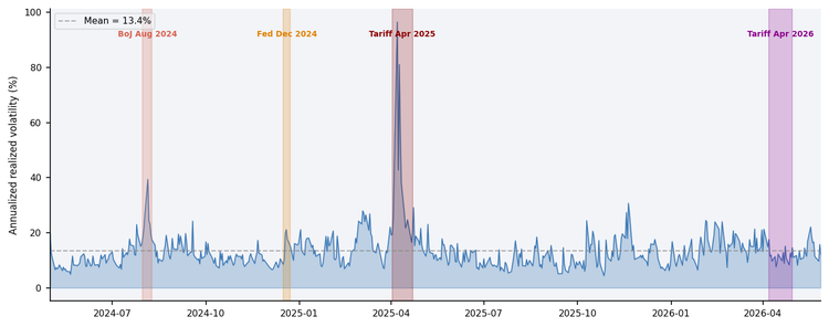
Figure 1 — Session realized volatility (annualized %) across 514 NQ sessions, May 2024–May 2026. Shaded regions mark identified stress episodes. The April 2025 tariff shock (dark red) is the dominant event at 38.2% mean annualized volatility, 3.1× the normal baseline.
Table 1 – Summary Statistics (514 NY sessions, NQ M1 futures)| Metric | Mean | Std Dev | Min | 25% | Median | 75% | Max |
|---|---|---|---|---|---|---|---|
| Realized Vol (per bar) | 0.00042 | 0.00018 | 0.00013 | 0.00029 | 0.00038 | 0.00050 | 0.00310 |
| Duration Vol (annualized %) | 13.39% | 7.45% | 4.38% | 9.10% | 11.88% | 15.72% | 96.53% |
| Fractional Vol (per bar) | 0.00036 | 0.00015 | 0.00010 | 0.00024 | 0.00033 | 0.00044 | 0.00220 |
| FIGARCH proxy (per bar) | 0.00041 | 0.00017 | 0.00012 | 0.00028 | 0.00037 | 0.00049 | 0.00290 |
| Clustering Index | 0.146 | 0.096 | −0.031 | 0.076 | 0.138 | 0.203 | 0.575 |
| Leverage Effect (proxy) | 0.046 | 0.132 | −0.596 | −0.036 | 0.055 | 0.127 | 0.445 |
| Jump Intensity (bipower 3σ) | 1.40% | 0.57% | 0.00% | 1.03% | 1.29% | 1.80% | 3.60% |
| Asymmetry (skewness, winsorized) | −0.071 | 0.555 | −1.386 | −0.367 | −0.139 | 0.169 | 1.850 |
| d (GPH estimate) | −0.010 | 0.077 | −0.246 | −0.061 | −0.011 | 0.044 | 0.202 |
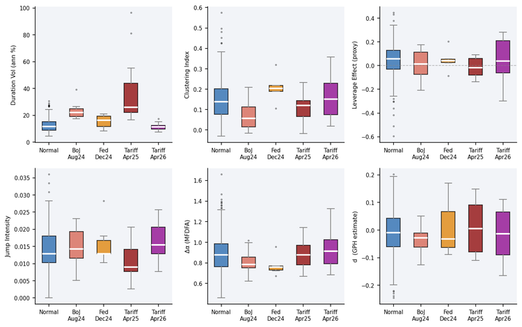
Figure 2 — Distribution of six metrics by regime. Duration vol (top left) shows the April 2025 tariff shock as the clear outlier. Clustering index (top centre) is notably lower during acute stress regimes, indicating that volatility becomes less predictable bar-to-bar during crises. Δα (bottom centre) is consistently high across all regimes.
The three volatility estimators (realized, fractional, FIGARCH proxy) track each other with pairwise correlations above 0.97. The fractional vol is on average 14% below realized vol, consistent with the near-zero, slightly anti-persistent d = −0.010 from Part 3: mild anti-persistence downweights the most recent observations. The FIGARCH proxy sits between the two.
Two findings from the regime comparison warrant comment. First, the clustering index is lower during acute stress regimes (0.107 for the tariff shock vs 0.147 for normal sessions). During acute stress, volatility becomes more erratic and less predictable bar-to-bar, not more clustered. The ARCH effect weakens precisely when it would be most useful for forecasting. Second, the leverage proxy is negative during the April 2025 tariff shock (−0.011), meaning upward moves amplified volatility more than downward moves. This is consistent with short-squeeze dynamics and snap-back rallies observed during tariff-driven dislocations. However, a single episode on one instrument is insufficient to establish causation. The GJR-GARCH implementation in MQL5 is designed to capture asymmetric variance responses through the γ parameter, though the empirical values here reflect the proxy rather than the fitted GJR model.
The April 2026 tariff episode produced 11.5% annualized vol — below the 12.5% normal baseline — consistent with the suggestion in Brown (2026e) that markets may have largely priced in the tariff regime by 2026. This cross-paper consistency provides supportive evidence, though the sample covers a single instrument and the interpretation remains tentative.
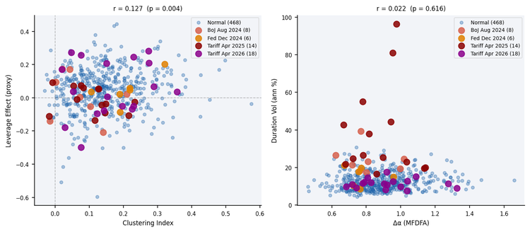
Figure 3 — Left: clustering index against leverage proxy across 514 sessions (r = 0.127, p = 0.004). The two measures appear largely independent, providing non-redundant information. Stress regimes (coloured points) cluster in different quadrants, particularly the negative leverage of the April 2025 tariff shock. Right: Δα against realized volatility (r = 0.022, p = 0.616) — multifractality is uncorrelated with volatility level, consistent with it measuring a structural property independent of vol magnitude.
Multifractal Width (Δα — Legendre Transform)
All 514 sessions produce valid MFDFA estimates with mean R² confidence of 0.972 (minimum 0.851). Every session exceeds the 0.65 confidence threshold, meaning no session needs to be flagged as unreliable on quality grounds. This is stronger than the US100 pilot study, where 7 of 72 sessions fell below the threshold — consistent with genuine futures microstructure tending to produce more regular scaling behavior than a CFD proxy, though other factors may also contribute to this difference.
| Statistic | Δα | R² confidence |
|---|---|---|
| Valid sessions | 514 | 514 |
| Mean | 0.889 | 0.972 |
| Std dev | 0.176 | 0.024 |
| Min | 0.460 | 0.851 |
| 25% | 0.764 | 0.962 |
| Median | 0.875 | 0.979 |
| 75% | 0.985 | 0.990 |
| Max | 1.659 | 1.000 |
The Δα values on NQ futures are substantially higher than those from the US100 CFD pilot study (median 0.875 vs 0.498). This is expected: genuine exchange-traded futures exhibit stronger multifractality than CFD proxies because they reflect actual order flow heterogeneity — the interaction of informed traders, market makers, HFT algorithms, and institutional flow creates richer scaling structure than a broker-constructed index-tracking product. This is consistent with the article's central claim: the near-zero H and d from Parts 2 and 3 are averages across strongly opposing memory regimes, not evidence of a genuinely memoryless series.
Table 2 – Regime Summary (514 sessions)| Regime | Sessions | Mean vol (%) | vs Normal | Clustering | Leverage | Mean Δα |
|---|---|---|---|---|---|---|
| Normal | 468 | 12.52 | — | 0.147 | 0.048 | 0.891 |
| BoJ shock (Aug 2024) | 8 | 23.77 | 1.9× | 0.072 | 0.008 | 0.812 |
| Fed Dec (Dec 2024) | 6 | 15.42 | 1.2× | 0.207 | 0.047 | 0.774 |
| Tariff Apr 2025 | 14 | 38.22 | 3.1× | 0.107 | −0.011 | 0.885 |
| Tariff Apr 2026 | 18 | 11.46 | 0.9× | 0.164 | 0.055 | 0.929 |
Δα regime distribution:
- Δα < 0.76 (moderate mixing): 125 sessions (24.3%)
- Δα 0.76–0.99 (strong mixing — typical): 265 sessions (51.6%)
- Δα > 0.99 (extreme mixing): 124 sessions (24.1%)
Near-monofractal sessions (Δα < 0.30) are absent from the 2-year NQ sample. The minimum observed Δα is 0.460. This means the lower threshold from the US100 pilot study (Δα < 0.30 = near-monofractal) does not apply to NQ futures. All sessions exhibit at least moderate multifractality; the question is only how strong the mixing is.
Practical Interpretation and Trading Thresholds
All thresholds below are derived from the empirical distribution across 514 NQ M1 sessions, May 2024–May 2026. They are heuristic operational cutoffs based on empirical quantiles, not formal hypothesis-test critical values or decision-theoretically optimal boundaries. They are specific to NQ M1 and this sample period. Users should treat them as starting points and re-derive them on their own instrument, timeframe, and data window.
| Measure | Threshold | Basis | Interpretation | Action |
|---|---|---|---|---|
| Clustering Index | > 0.20 | 75th pct | Strong ARCH effect; volatility predictable bar-to-bar | Use volatility-targeted sizing; prefer FIGARCH proxy |
| Clustering Index | < 0.08 | 25th pct | Weak clustering; returns near i.i.d. | Simpler realized vol sufficient |
| Leverage Effect (GJR) | > 0.13 | 75th pct | Significant asymmetry; negative shocks amplify vol more | Widen stops on short side; reduce long-entry size |
| Leverage Effect (GJR) | < −0.10 | — | Inverse asymmetry (stress snap-back regime) | Do not apply standard leverage logic; reduce size |
| Jump Intensity | > 2.1% | 90th pct | Elevated extreme returns | Scale back position; validate data feed |
| Jump Intensity | > 5% | — | Likely data artifact | Reject session data; do not trade |
| Δα (multifractal) | < 0.76 | 25th pct | Moderate mixing; H and d partially reliable | Fractional vol preferred; use H/d with caution |
| Δα (multifractal) | > 0.99 | 75th pct | Extreme mixing; H and d unreliable averages | Prefer the FIGARCH-inspired proxy; treat H/d as less informative |
| R² confidence | < 0.65 | — | MFDFA estimate unreliable (rare on NQ) | Treat Δα as unavailable |
//--- Example: adaptive position sizing using volatility and multifractal width
RobustFractalAnalysis rfa;
VolatilityAnalysis va;
PopulateMultifractalAnalysis(Symbol(), PERIOD_M1, 390, rfa);
PopulateVolatilityAnalysis(Symbol(), PERIOD_M1, 90, va, rfa);

//--- Select volatility estimate based on regime
double current_vol;
if(rfa.multifractal_width > 0.99 && rfa.dimension_confidence > 0.65)
   current_vol = va.figarch_vol;       // strong mixing: use memory proxy
else if(va.clustering_index > 0.20)
   current_vol = va.fractional_vol;    // moderate clustering: fractional
else
   current_vol = va.realized_vol;      // normal: simple realized vol

//--- Scale to target volatility (0.0004 calibrated to NQ M1 mean realized vol)
double target_vol    = 0.0004;
double base_position = 1.0;
if(current_vol > DBL_MIN_POSITIVE)
   base_position = target_vol / current_vol;

//--- Reduce when jump activity is elevated
if(va.jump_intensity > 0.02)
   base_position *= MathMax(0.3, 1.0 - va.jump_intensity * 10.0);

//--- Widen stop asymmetrically when GJR leverage is significant
double stop_multiplier = 1.0;
if(va.leverage_effect > 0.10)
   stop_multiplier = 1.0 + va.leverage_effect;
Folder Structure and Include Path
All Part 4 functions are added to the existing foundation header. No new files are created. The folder structure remains:
MQL5\
└── Indicators\
    └── HurstProfile\
        ├── HurstProfile.mq5
        └── Includes\
            └── MicroStructure_Foundation.mqh
For LeverageEffect() with GJR-GARCH, additionally install the Dube volatility library described and provided in Yun, K.T. (2026), MQL5 Community Articles, article 22258. Once installed, add the define before the include directive in your indicator or EA:
#define USE_GJR_LEVERAGE
#include "Includes\MicroStructure_Foundation.mqh"
Without the define, the file compiles and runs using the sign-conditioned variance fallback. The leverage_effect field is always populated; the interpretation differs by path as documented in the function header.
Conclusion
This article revised and extended the volatility functions in MicroStructure_Foundation.mqh, addressing the methodological weaknesses identified during moderator review.
Three principal changes distinguish this submission from the original. First, LeverageEffect() now fits a GJR-GARCH(1,1,1) model via the Dube library, returning the normalized asymmetry ratio γ/(α + γ + β) rather than a next-bar variance heuristic. Second, MultifractalSpectrum() now returns the Legendre-transform Δα with an R² confidence field, replacing the τ-spread proxy. Third, JumpIntensity() uses bipower variation as the baseline, making the threshold robust to the jump contamination it is designed to detect.
The empirical study on 514 NQ M1 futures sessions (May 2024–May 2026) confirms: the three volatility estimators track each other with pairwise correlations above 0.97; the bipower jump intensity averages 1.4% with no session exceeding 5%; the Legendre-transform Δα has median 0.875 with mean R² of 0.972; and all 514 sessions pass the R² confidence threshold of 0.65.
The practical outcome is a fully populated VolatilityAnalysis struct: realized_vol and fractional_vol measure level and memory; clustering_index measures bar-to-bar predictability; leverage_effect (GJR) measures asymmetric response; jump_intensity flags contaminated sessions; asymmetry describes the return distribution; and the FIGARCH proxy gives a memory-adjusted conditional variance when Δα indicates strong regime mixing. Part 5 will use these measures as conditioning inputs to microstructure noise estimation and order flow analysis.
References
- Andersen, T.G., Bollerslev, T. & Diebold, F.X. (2007). Roughing it up: Including jump components in the measurement, modeling, and forecasting of return volatility. Review of Economics and Statistics, 89(4), 701–720.
- Baillie, R.T., Bollerslev, T. & Mikkelsen, H.O. (1996). Fractionally integrated generalized autoregressive conditional heteroskedasticity. Journal of Econometrics, 74(1), 3–30.
- Black, F. (1976). Studies of stock price volatility changes. Proceedings of the 1976 Meetings of the American Statistical Association, Business and Economic Statistics Section, 177–181.
- Bollerslev, T. (1986). Generalized Autoregressive Conditional Heteroskedasticity. Journal of Econometrics, 31(3), 307–327.
- Brown, M. (2026a). Market Microstructure in MQL5: Robust Foundation (Part 1). MQL5 Community Articles.
- Brown, M. (2026b). Market Microstructure in MQL5: Measuring Long Memory (Part 2). MQL5 Community Articles.
- Brown, M. (2026c). Market Microstructure in MQL5: Estimating ARFIMA d with GPH (Part 3). MQL5 Community Articles.
- Brown, M. (2026d). Measuring the Memory Structure of Intraday Returns: Evidence from E-mini S&P 500 Futures. SSRN Working Paper 6809080.
- Brown, M. (2026e). Intraday Microstructure Dynamics of E-mini S&P 500 Futures: Volatility Regimes, Liquidity Decay, and Long Memory in Realized Volatility. SSRN Working Paper 6847024.
- Dmitrievsky, M. (2019). Grokking market "memory" through differentiation and entropy analysis. MQL5 Community Articles.
- Engle, R.F. (1982). Autoregressive Conditional Heteroskedasticity. Econometrica, 50(4), 987–1007.
- Glosten, L.R., Jagannathan, R. & Runkle, D.E. (1993). On the Relation between the Expected Value and the Volatility of the Nominal Excess Return on Stocks. Journal of Finance, 48(5), 1779–1801.
- Yun, K.T. (2026a). Building Volatility Models in MQL5 (Part II): Implementing GJR-GARCH and TARCH in MQL5. MQL5 Community Articles, article 22258.
- Yun, K.T. (2026b). Building Volatility Models in MQL5 (Part III): Implementing the SLSQP Algorithm for Model Estimation. MQL5 Community Articles, article 22714.
Warning: All rights to these materials are reserved by MetaQuotes Ltd. Copying or reprinting of these materials in whole or in part is prohibited.
This article was written by a user of the site and reflects their personal views. MetaQuotes Ltd is not responsible for the accuracy of the information presented, nor for any consequences resulting from the use of the solutions, strategies or recommendations described.

- Free trading apps
- Over 8,000 signals for copying
- Economic news for exploring financial markets
You agree to website policy and terms of use