Elements of correlation analysis in MQL5: Pearson chi-square test of independence and correlation ratio

Introduction

In this article, I would like to touch upon such an important section of mathematical statistics as correlation analysis, including the detection and evaluation of dependencies between random variables. The most popular tool in the arsenal of correlation analysis is, of course, the correlation ratio. However, calculating the correlation ratio alone is completely insufficient if we want to assess dependencies in data, especially such as stock price increments. First, the ratio only evaluates linear dependence. Second, zero values of the correlation ratio do not mean the absence of dependence if the data sample it is calculated from has a distribution different from the normal one. To answer the question of whether the data are dependent, we should define the independence criteria. We will talk about the most famous criterion - Pearson's chi-square test of independence. We will also talk about such a numerical characteristic as the correlation ratio, which helps to determine whether the dependence under study is non-linear.

Independence hypothesis

It is assumed that the data represent observations of some two-dimensional random variable (X, Y) with an unknown distribution function F(X, Y), about which it is required to test the independence hypothesis H0 : F(X, Y) = F(X)*F(Y), where F(X) and F(Y) are one-dimensional distribution functions.

By X and Y random variables in this article I will mean either increments of the logarithms of prices of different financial instruments, or increments of the prices of one instrument taken with the lag of one.

Pearson chi-square test of independence

The chi-square independence criterion is used both for discrete random variables with a finite number of outcomes and for continuous random variables, but with the obligatory condition of their preliminary grouping. In this case, the set of all possible values of the random X variable is divided into i non-intersecting intervals A1, A2, Ai, and the set of all Y values is divided into a set of j non-intersecting intervals B1, B2, Bj. Thus, the set of values of a two-dimensional quantity (X, Y) is divided into i*j rectangles (cells). For clarity, these data are presented in the form of a so-called feature contingency table (correlation table, probability distribution table of a two-dimensional random variable, etc.).

                              

In the table:

• Ai = (Xi-1, Xi) - i th interval of a random X value grouping

• Bj = (Yj-1,Yj) – j th interval of a random Y value grouping

• nij - cell actual group frequency (number of those pairs of observations (X, Y) whose values fall within the Ai and Bj interval)

• ni. - number of observations in the i th row

• n.j – number of observations in the j th column

• N – sample volume

The following statistic is used as chi-square test of independence:

CHI2 = (Actual – Expected) ^2 / Expected,

where

• Actual - nij cell actual group frequency,

• Expected – nij cell expected group frequency

These statistics are chi-square distributed with v = (j-1)(i-1) degrees of freedom.

The null hypothesis of independence is rejected if the estimated CHI2 statistic exceeds the critical values of the chi-square distribution with v degrees of freedom at some 'alpha' significance level.

We will calculate the actual frequencies based on the sample data. The principle for constructing the expected frequencies is as follows: if the random variables X and Y are independent, then the following equation is valid:

P {Ai, Bj} = P {Ai}*P{Bj},

in other words, the probability of the simultaneous occurrence of Ai and Bj events is equal to the product of the probability of the Ai events occurrence and the probability of the Bj event occurrence.

To find the mathematical expectations of {Ai, Bj}, {Ai} and {Bj} events, multiply both parts of this equality by N*N, that is, by the square of the number of observations.

N*N * P {Ai, Bj} = N *P{Ai} * N* P{Bj}

Then we get:

• N *P{Ai} - mathematical expectation of the number of observations in the i th row

• N* P{Bj} - mathematical expectation of the number of observations in the j th column

• N * P {Ai, Bj} = (N *P{Ai} * N* P{Bj})/N - mathematical expectation of the number of cell hits at the intersection of the i th row and j th column

Then, substituting ni and n.j estimates instead of N *P{Ai} and N* P{Bj} mathematical expectations (the actual frequencies from the correlation table), we obtain the desired estimate of the expected frequencies

Expected = (ni. * n.j)/N

Thus, according to the independence hypothesis, the expected frequency of hitting a cell at the intersection of the i-th row and the j-th column is equal to the product of the sums of the number of observations in the i th row and the j th column divided by the sample size.

Therefore, when calculating the criterion, it is natural to expect that the more the actual frequencies differ from the expected ones, the greater the likelihood that the data are not independent.

Chi2Test indicator

Pearson chi-square independence test calculation is implemented in the Chi2Test indicator. The indicator tests the independence hypothesis on each bar between adjacent price increments for a single financial instrument.

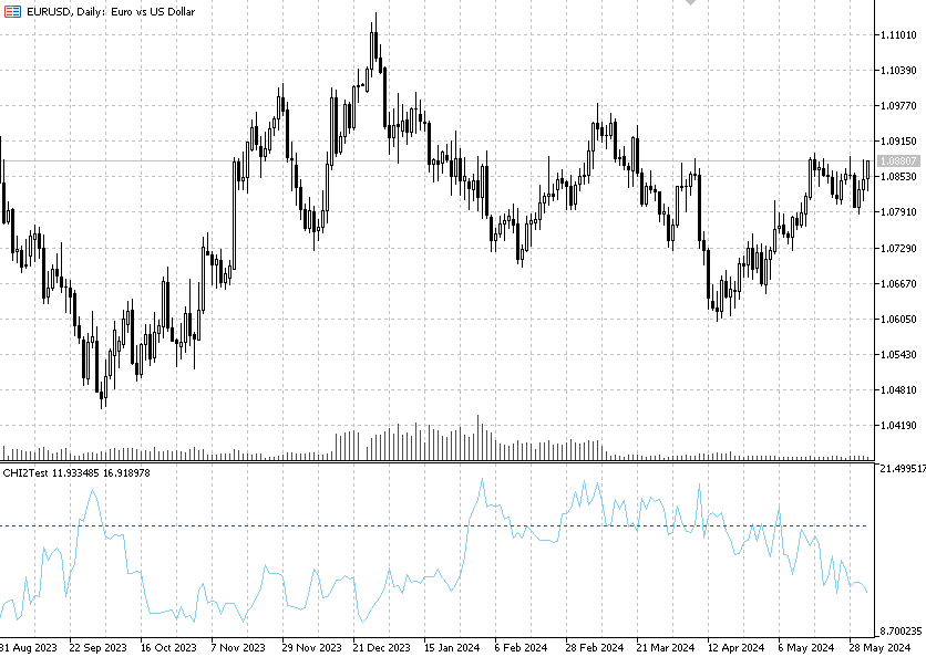
The indicator has four inputs:

• alpha – significance level

• Data – data window for calculation

• Tails - number of standard deviations

• Contingency coefficient

In order to calculate the chi-square statistic, we first need to calculate the actual frequencies in the feature contingency table. This is done by the crosstab function.

//+------------------------------------------------------------------+
//|  Calculate the table of contingency of two random values (X,Y)   |
//+------------------------------------------------------------------+
bool Crosstab(const double &dataX[],const double &dataY[],const double &bins[],matrix &freq)
  {

   int datasizeX=ArraySize(dataX);
   int datasizeY=ArraySize(dataY);
   int binssize=ArraySize(bins);
   if(datasizeX==0 || datasizeY==0 || binssize==0)
      return(false);
   if(datasizeX != datasizeY)
      return(false);

   for(int i=0; i<datasizeX; i++)
     {
      if(!MathIsValidNumber(dataX[i]) || !MathIsValidNumber(dataY[i]))
         return(false);
     }

   matrix m_freq=matrix::Zeros(binssize, binssize);
   
   for(int x=0; x<binssize; x++)
     {
      for(int i=0; i<datasizeX; i++)
        {
         for(int y=0; y<binssize; y++)
           {
            if(dataX[i]<=bins[x] && dataY[i]<=bins[y]) 
              {
               m_freq[x,y]=m_freq[x,y]+1;
               break;
              }
           }
        }
     }
     
   matrix Actual = m_freq;
   vector p1,p2,diffp;
   for (int j=1; j<binssize; j++)
   {
   p1 = m_freq.Row(j-1);
   p2 = m_freq.Row(j);
   diffp = p2-p1;
   Actual.Row(diffp,j);   
   }
   freq = Actual; 
   
   return(true);
  }

Since the data we are working with is continuous, the first thing we need to do is group it. In this case, we can find recommendations stating that in order to calculate the test correctly, it is desirable for the minimum value of the expected frequency in the cells to be not less than one, while the number of the cells, in which the expected frequency is less than five, should not be large (for example, two such cells are allowed if the total number of cells is less than 10). Since stock data distributions have heavy tails, a certain difficulty arises in constructing grouping intervals that can meet the above requirements.

I propose to group the data after standardizing it. After that, trim the heavy tails of the distribution to 2-3-4 sigma, depending on the volume of data being analyzed. In the indicator, this is done by the Tails parameter. For example, if the data volume is small (200-300 values), then we should choose the Tails value equal to 2 sigma. As a result, we get grouping intervals: (-2,-1), (-1,0), (0,1), (1,2) and, consequently, a 4x4 feature contingency table. Thus, we will combine adjacent grouping intervals with small expected frequencies in order to correctly calculate the chi-square statistic.

Cramer's contingency coefficient

Unfortunately, the CHI2 statistic cannot serve as a numerical measure of probability dependence, so Cramer's contingency coefficient is used for this purpose. Its values vary from zero to one. Zero means no dependency between data, one means functional dependency.

Cramer's contingency coefficient is based on the chi-square statistic:

Contingency coefficient = sqrt (CHI2 / N*(Bins_count-1)),

where Bins_count is a number of rows (or columns) in the feature contingency table.

Thus, two statistics are in fact implemented in a single indicator – the main chi-square statistic and the contingency coefficient calculated on its basis.

If you want to test the independence of two different financial instruments, use the Crosstab script. To do this, activate the X vs Y (true) parameter. Otherwise, the script calculates statistics based on the current symbol data. Sample data for calculation is counted from the penultimate bar on the chart.

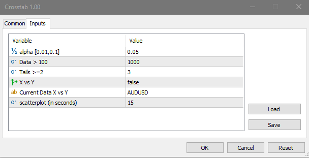
Crosstab script calculates and logs the following information:

• matrix of actual (Actual ) and expected (Expected) frequencies

• r correlation ratio calculated by grouped data

• Pearson correlation ratio calculated from ungrouped data (in order to compare the accuracy of calculations, since statistics calculated from grouped data are less accurate)

• Nxy, Nyx (Correlation ratio) correlation ratio

• results of testing the hypothesis of the absence of correlation dependence (f statistic correl independence)

• results of testing the hypothesis of the correlation dependence linearity (f statistic Linear/Nonlinear),

• CHI2 chi-square statistics

• Cramer's contingency coefficient

A scatterplot diagram (correlation field) is also displayed on the screen for visual assessment of the pair dependence.

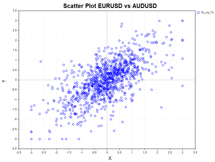
Use the Crosstab_Models script to test model data for independence. The models used are uniform distribution, first-order auto regression, ARCH auto regressive conditional heteroscedasticity and logistic mapping.

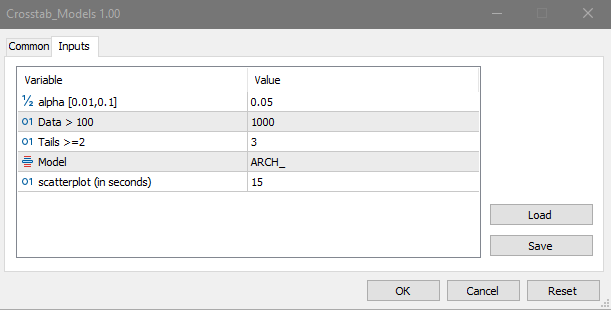
Model data serves as a kind of a template used to compare results obtained from real data. For example, this is what a non-linear dependence looks like in a one-dimensional non-linear dynamic system - a logistic mapping:

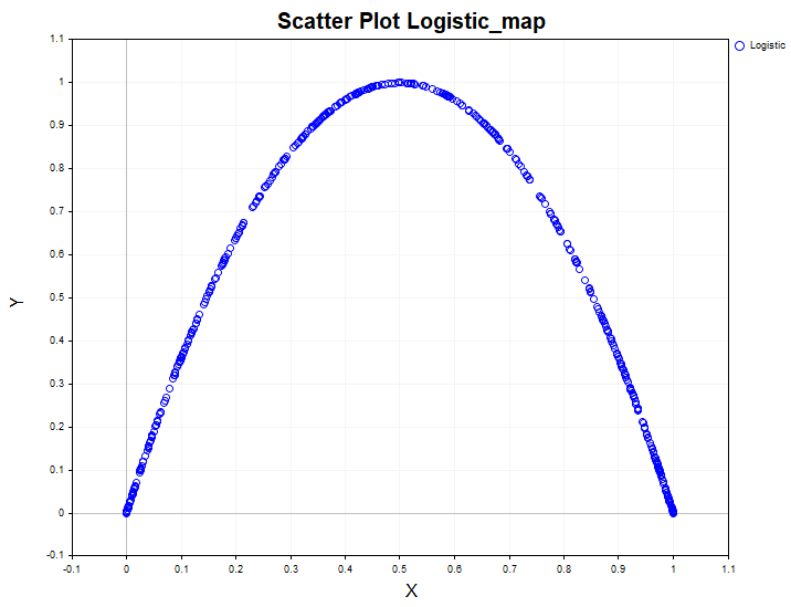
By analyzing the data of such a system using only the linear correlation ratio, one could erroneously conclude that this process is white noise. At the same time, the chi-square independence test easily reveals that the data are dependent, and the correlation ratio confirms that the dependence is non-linear.

Correlation ratio

The correlation ratio is used to assess the non-linearity of the correlation dependence:

Nyx = sqrt (D[E(Y|X)]/Sy)

Nxy = sqrt (D[E(X|Y)])/Sx)

where:

• E(Y|X) — conditional mathematical expectation of the Y random value

• E(X|Y) — conditional mathematical expectation of the X random value

• D[E(Y|X)] – conditional mathematical expectation variance of the Y random value

• D[E(X|Y)] – conditional mathematical expectation variance of the X random value

• Sy, Sx – unconditional variances of Y and X random values

Let us remember that:

• E(Y|X) conditional mathematical expectation is a random value.

• E[E(Y|X)] = E[Y] (mathematical expectation of the Y random value unconditional mathematical expectation is equal to the Y unconditional mathematical expectation).

• Y dispersion is D[Y] = E[(Y – E(Y) )^2)] mathematical expectation of the square of the Y random value deviation from the E[Y] mathematical expectation.

• Then D[E(Y|X)] = E{[ E(Y|X) – E[Y] ] ^ 2}. In other words, the E(Y|X) unconditional mathematical expectation variance is equal to the mathematical expectation of the square of the E(Y|X) unconditional mathematical expectation deviation from the E[Y] unconditional mathematical expectation.

In other words, the correlation ratio is the square root of the ratio of two variances - conditional and unconditional one. The correlation ratio can only be calculated based on the correlation table, that is, based on grouped data. Let's list the properties it has:

• the correlation ratio is asymmetric with respect to X and Y, that is, Nxy != Nyx.

• 0 ≤ | r | ≤ Nxy ≤ 1, 0 ≤ | r | ≤ Nyx ≤ 1, the values of the indicator lie within the range [0,1] and are always greater than or equal to the r correlation linear ratio, which is taken modulo.

• if the data are independent, then Nxy=Nyx=0. The converse is not true, that is, uncorrelatedness does not imply independence.

• if | r | = Nyx =Nyx <1, then the correlation between X and Y is linear, that is, no better curve than a straight line can be found for the regression equation.

• if the correlation between X and Y is non-linear, then | r | < min (Nxy, Nyx). The smaller the difference between the correlation ratio and the correlation relationship, the closer the relationship between X and Y to the linear one.

By calculating the sample correlation relationship, we can check the hypothesis of the absence of a correlation between two random variables (H0: Nyx = 0).

To do this, the following statistics are calculated:

F = Nyx^2 * (N-Bins_count) / (1- Nyx^2) *(Bins_count-1)

If the tested hypothesis is true, the F statistic is distributed according to Fisher's law with v1 = Bins_count-1 and v2 = N-Bins_count degrees of freedom.

The null hypothesis is rejected at the alpha significance level if the calculated value of the F statistic exceeds the critical value of this statistic (then the alternative H1 is accepted: Nyx >0)

Let's say we are convinced that the correlation dependence is present. The question arises: is this dependence linear or non-linear? The hypothesis about the linearity of the correlation dependence between two random variables answers this question.

When testing the hypothesis about the linearity of the correlation dependence of Y on X (H0: Nyx^2 = r^2), the following statistics is used:

F = (Nyx^2 - r^2) * (N-Bins_count) / (1- Nyx^2) *(Bins_count-2)

If the tested hypothesis is true, the F statistic is distributed according to Fisher's law with v1= Bins_count-2 and v2 = N-Bins_count degrees of freedom.

The null hypothesis about correlation linearity is rejected at the alpha significance level if the calculated value of the F statistic exceeds the critical value of this statistic (then the alternative H1 is accepted: Nyx^2 != r^2 )

Conclusion

The article examined such important tools of correlation analysis as Pearson's chi-square test of independence and the correlation ratio. With their help, it is possible to assess the presence of hidden relationships in the data much more accurately. The CHI2Test indicator tests the hypothesis of independence, allowing us to obtain statistically valid conclusions about the presence of relationships in the data.

in addition to the chi-square statistics, the Crosstab and Crosstab_Models scripts also calculate the correlation ratio and test the hypothesis about the correlation dependence and the linearity of this dependence, including for model data. Additionally, a correlation field graph is displayed on the screen for visual assessment of the pair dependence. The user can regulate the accuracy of statistical tests by choosing the desired alpha significance level. The lower the significance level, the less likely it is to get a false answer.