Training a multilayer perceptron using the Levenberg-Marquardt algorithm

Introduction

The purpose of this article is to provide practicing traders with a very effective neural network training algorithm - a variant of the Newtonian optimization method known as the Levenberg-Marquardt algorithm. It is one of the fastest algorithms for training feed-forward neural networks, rivaled only by the Broyden-Fletcher-Goldfarb-Shanno (L-BFGS) algorithm.

Stochastic optimization methods such as stochastic gradient descent (SGD) and Adam are well suited for offline training when the neural network overfits over long periods of time. If a trader using neural networks wants the model to quickly adapt to constantly changing trading conditions, he needs to retrain the network online at each new bar, or after a short period of time. In this case, the best algorithms are those that, in addition to information about the gradient of the loss function, also use additional information about the second partial derivatives, which allows finding a local minimum of the loss function in just a few training epochs.

At the moment, as far as I know, there is no publicly available implementation of the Levenberg-Marquardt algorithm in MQL5. It is time to fill this gap, and also, at the same time, briefly go over the well-known and simplest optimization algorithms, such as gradient descent, gradient descent with momentum, and stochastic gradient descent. At the end of the article, we will conduct a small test of the efficiency of the Levenberg-Marquardt algorithm and algorithms from the scikit-learn machine learning library.

Dataset

All subsequent examples use synthetic data for ease of presentation. Time is used as the only predictor variable, and the target variable that we want to predict using the neural network is the function:

1 + sin(pi/4*time) + NormDistr(0,sigma)

This function consists of a deterministic part, represented by a periodic component in the form of a sine, and a stochastic part - Gaussian white noise. Total 81 data points. Below is a graph of this function and its approximation by a three-layer perceptron.

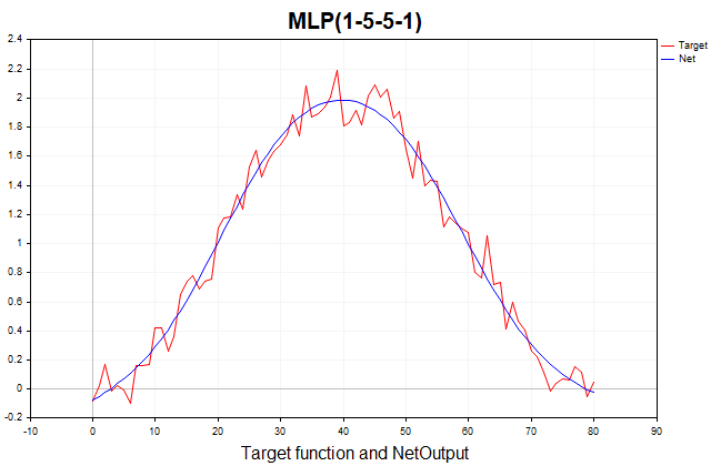
Fig. 1. The target function and its approximation by a three-layer perceptron

Gradient descent

Let's start with the implementation of the regular gradient descent, as the simplest method for training neural networks. I will use a very good example from the MQL5 Reference book as a template (Matrix and Vector Methods/Machine learning). I modified it a bit, adding the ability to select the activation function for the last layer of the network and making the implementation of gradient descent universal, capable of learning not only on the quadratic loss function, as implicitly assumed in the example from the reference book, but on all available loss functions in MQL5. The loss function is central to training neural networks, and it is sometimes worth experimenting with different functions beyond just the quadratic loss. Here is the general equation for calculating the output layer error (delta):

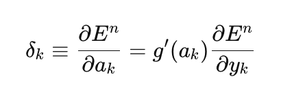
here

• delta_k — output layer error,
• E — loss function,
• g'(a_k) — derivative of the activation function,
• a_k — pre-activation of the last layer,
• y_k — predicted value of the network.

//--- Derivative of the loss function with respect to the predicted value       
matrix DerivLoss_wrt_y = result_.LossGradient(target,loss_func);  
matrix deriv_act;
  if(!result_.Derivative(deriv_act, ac_func_last)) 
     return false;      
 matrix  loss = deriv_act*DerivLoss_wrt_y;  // loss = delta_k

The partial derivatives of the loss function with respect to the predicted value of the network are calculated by the LossGradient function, while the derivative of the activation function is calculated by the Derivative function. In the reference example, the difference between the target and predicted value of the network multiplied by 2 is used as the error of the output layer.

matrix loss = (target - result_)*2; 

In the machine learning literature, the error of each layer of the network is usually called delta(D2,D1 etc.) rather than loss (for example, see Bishop(1995)). From now on, I will use exactly this notation in the code.         

How did we get this result? Here, it is implicitly assumed that the loss function is the sum of squared differences between the target and predicted values, rather than the mean squared error (MSE), which is additionally normalized by the size of the training sample. The derivative of this loss function is exactly equal to (target - result)*2. Since the last layer of the network uses the identical activation function, whose derivative is equal to one, we arrive at this result. Therefore, those who want to use arbitrary loss functions and output layer activation functions to train the network need to use the above general equation.

Let's now train our network on the mean square loss function. Here, have displayed the graph on a logarithmic scale for clarity.

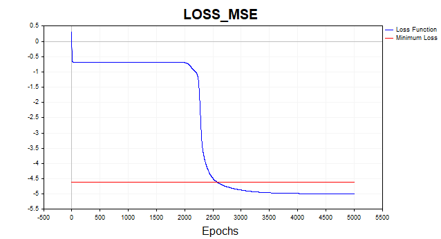
Fig. 2. MSE loss function, gradient descent

On average, the gradient descent algorithm requires 1500-2000 epochs (i.e. passes over the entire training data set) to reach the minimum loss function threshold. In this case, I used two hidden layers with 5 neurons in each.

The red line on the graph indicates the minimum threshold of the loss function. It is defined as the variance of white Gaussian noise. Here I used noise with variance equal to 0.01 (0.1 sigma* 0.1 sigma).

What happens if we allow the neural network model to learn below this minimum threshold? Then we will encounter such an undesirable phenomenon as network overfitting. It is pointless to try to get the loss function error on the training dataset below the minimum threshold, as this will affect the predictive power of the model on the test dataset. Here we are faced with the fact that it is impossible to predict a series more accurately than the statistical spread of that series allows. If we stop training above the minimum threshold, we will face another problem - the network will be undertrained. That is, one that was unable to fully capture the predictable component of the series.

As you can see, gradient descent needs to go through quite a few iterations to reach the optimal set of parameters. Note that our dataset is pretty simple. For real practical problems, the training time for gradient descent turns out to be unacceptable. One of the simplest ways to improve the convergence and speed of gradient descent is the momentum method.

Gradient descent with momentum

The idea behind gradient descent with momentum is to smooth out the trajectory of the network parameters during training by averaging the parameters like a simple exponential average. Just as we smooth the time series of prices of financial instruments with an average in order to highlight the main direction, we also smooth the trajectory of a parametric vector that moves toward the point of a local minimum of our loss function. To better visualize this, let's look at a graph that shows how the values of the two parameters changed - from the beginning of training to the minimum point of the loss function. Fig. 3 shows the trajectory without using momentum. 

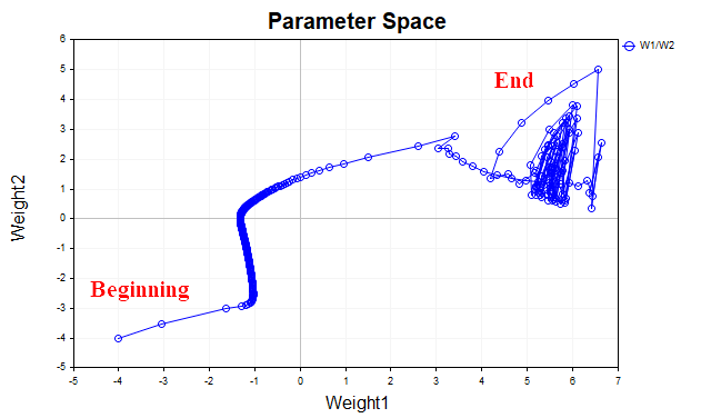
Fig. 3. Gradient descent without momentum

We see that as the minimum approaches, the parameter vector begins to oscillate chaotically, which does not allow us to reach the optimum point. To get rid of this phenomenon, we will have to reduce the learning rate. Then the algorithm will, of course, begin to converge, but the time spent on the search may increase significantly.

Fig. 4 shows the trajectory of the parameter vector using the moment (with the value of 0.9). This time the trajectory is smoother, and we easily reach the optimum point. Now we can even increase the learning rate. This is, in fact, the main idea of gradient descent with momentum - to speed up the convergence process.

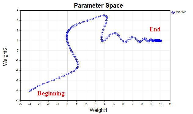
Fig. 4. Gradient descent, momentum (0.9)

The Momentum_SD script implements the gradient descent algorithm with momentum. In this algorithm, I decided to get rid of one hidden layer and separate the weights and biases of the network, for clarity of perception. Now we have only one hidden layer with 20 neurons instead of two hidden layers with 5 neurons each, as in the previous example.

//+------------------------------------------------------------------+
//|                                                  Momentum_SD.mq5 |
//|                                                           Eugene |
//|                                             https://www.mql5.com |
//+------------------------------------------------------------------+
#property copyright "Eugene"
#property link      "https://www.mql5.com"
#property version   "1.00"
#property script_show_inputs
#include <Graphics\Graphic.mqh>
#include <Math\Stat\Math.mqh>
#include <Math\Stat\Normal.mqh>
enum Plots
  {
   LossFunction_plot,  
   target_netpredict_plot
  };
  
matrix weights1, weights2,bias1,bias2;                      // network parameter matrices
matrix dW1,db1,dW2,db2;                                     // weight increment matrices
matrix n1,n2,act1,act2;                                     // neural layer output matrices
input int    layer1                  = 20;                  // neurons Layer 1
input int    Epochs                  = 1000;                // Epochs
input double lr                      = 0.1;                 // learning rate coefficient
input double sigma_                  = 0.1;                 // standard deviation synthetic data
input double gamma_                  = 0.9;                 // momentum 
input Plots  plot_                   = LossFunction_plot;   // display graph
input bool   plot_log                = false;               // Plot Log graph
input ENUM_ACTIVATION_FUNCTION ac_func      = AF_TANH;      // Activation Layer1
input ENUM_ACTIVATION_FUNCTION ac_func_last = AF_LINEAR;    // Activation Layer2
input ENUM_LOSS_FUNCTION       loss_func    = LOSS_MSE;     // Loss function

double LossPlot[],target_Plot[],NetOutput[];
matrix ones_;
int Sample_,Features; 

//+------------------------------------------------------------------+
//| Script start function                                            |
//+------------------------------------------------------------------+
void OnStart()
  {
//--- generate a training sample
   matrix data, target;
   Func(data,target);
   StandartScaler(data);
   Sample_= (int)data.Rows();
   Features = (int)data.Cols();
   ArrayResize(target_Plot,Sample_);
   for(int i=0; i< (int)target.Rows(); i++)
     {
      target_Plot[i] =target[i,0];
     }
   ones_ = matrix::Ones(1,Sample_);  
      
   ulong start=GetMicrosecondCount(); 
//--- train the model
   if(!Train(data, target, Epochs))
      return;
   ulong end = (GetMicrosecondCount()-start)/1000;  
   Print("Learning time = " + (string)end + " msc");
//--- generate a test sample
    Func(data,target);
    StandartScaler(data);
//--- test the model
   Test(data, target);
//--- display graphs  
   PlotGraphic(15,plot_log);
  }
//+------------------------------------------------------------------+
//| Model training method                                            |
//+------------------------------------------------------------------+
bool Train(matrix &data, matrix &target, const int epochs)
  {
//--- create the model
   if(!CreateNet())
      return false;
   ArrayResize(LossPlot,Epochs);
//--- train the model
   for(int ep = 0; ep < epochs; ep++)
     {
      //--- feed forward
      if(!FeedForward(data))
         return false;
      PrintFormat("Epoch %d, loss %.5f", ep, act2.Loss(target, loss_func));
      LossPlot[ep] = act2.Loss(target, loss_func);
      //--- backpropagation and update of weight matrix
      if(!Backprop(data, target))
         return false;
     }
//---
   double rmse=act2.RegressionMetric(target.Transpose(),REGRESSION_RMSE);
   PrintFormat("rmse %.3f / sigma %.2f ",rmse,sigma_);
   ArrayResize(NetOutput,Sample_);
   for(int i=0; i< (int)act2.Cols(); i++)
     {
      NetOutput[i]  =act2.Transpose()[i,0];
     }
//--- return result
   return true;
  }
//+------------------------------------------------------------------+
//| Model creation method                                            |
//+------------------------------------------------------------------+
bool CreateNet()
  {
//--- initialize weight matrices
   if(!weights1.Init(layer1,Features)  || !weights2.Init(1,layer1)) 
      return false;
//--- initialize offset matrices
   if(!bias1.Init(layer1,1)  || !bias2.Init(1,1))  
      return false;
//--- initialize the matrix of parameter increments
   dW1.Init(layer1,Features);
   dW2.Init(1, layer1);
   db1.Init(layer1,1);
   db2.Init(1,1);
   dW1.Fill(0);
   dW2.Fill(0);
   db1.Fill(0);
   db2.Fill(0);
//--- fill the parameter matrices with random values
   weights1.Random(-0.1, 0.1);
   weights2.Random(-0.1, 0.1);
   bias1.Random(-0.1,0.1);
   bias2.Random(-0.1,0.1);
//--- return result
   return true;
  }
//+------------------------------------------------------------------+
//| Feed-forward method                                              |
//+------------------------------------------------------------------+
bool FeedForward(matrix &data)
  { 
//--- calculate the first neural layer
//--- n1 pre-activation of the first layer
   n1 = weights1.MatMul(data.Transpose()) + bias1.MatMul(ones_);
//--- calculate the activation function of the act1 first layer
   n1.Activation(act1, ac_func);
//--- calculate the second neural layer
//--- n2 pre-activation of the second layer
   n2 = weights2.MatMul(act1) + bias2.MatMul(ones_);
//--- calculate the activation function of the act2 second layer
   n2.Activation(act2, ac_func_last);
//--- return result
   return true;
  }
//+------------------------------------------------------------------+
//| Backpropagation method                                           |
//+------------------------------------------------------------------+
bool Backprop(matrix &data, matrix &target)
  {
//--- Derivative of the loss function with respect to the predicted value
   matrix DerivLoss_wrt_y = act2.LossGradient(target.Transpose(),loss_func);
   matrix deriv_act2;
   n2.Derivative(deriv_act2, ac_func_last);
//--- D2   
   matrix  D2 = deriv_act2*DerivLoss_wrt_y; // error(delta) of the network output layer
//--- D1
   matrix deriv_act1;
   n1.Derivative(deriv_act1, ac_func);
   matrix D1 = weights2.Transpose().MatMul(D2);
   D1 = D1*deriv_act1; // error (delta) of the first layer of the network
//--- update network parameters
   matrix  ones = matrix::Ones(data.Rows(),1);
   dW1 = gamma_*dW1 + (1-gamma_)*(D1.MatMul(data)) * lr;
   db1 = gamma_*db1 + (1-gamma_)*(D1.MatMul(ones)) * lr;
   dW2 = gamma_*dW2 + (1-gamma_)*(D2.MatMul(act1.Transpose())) * lr;
   db2 = gamma_*db2 + (1-gamma_)*(D2.MatMul(ones)) * lr;
   weights1 =  weights1 - dW1;
   weights2 =  weights2 - dW2;
   bias1    =  bias1    - db1;
   bias2    =  bias2    - db2;
//--- return result
   return true;
  }

Thanks to the momentum, I was able to increase the learning speed from 0.1 to 0.5. Now the algorithm converges in 150-200 iterations instead of 500 for regular gradient descent.

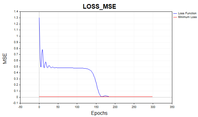
Fig. 5. MSE loss function, MLP(1-20-1) SD_Momentum

Stochastic gradient descent

Momentum is good, but when the data set is not 81 data points, as in our example, but tens of thousands of data instances, then it makes sense to talk about such a well-proven (and simple) algorithm as SGD. SGD is the same gradient descent, but the gradient is calculated not over the entire training set, but only on some very small part of this set (mini-batch), or even on one data point. After that, the network weights are updated, a new data point is randomly selected, and the process is repeated until the algorithm converges. That is why the algorithm is called stochastic. In conventional gradient descent, we updated the network weights only after we calculated the gradient on the entire data set. This is the so-called batch method.

We implement a variant of SGD where only one data point is used as a mini-batch.

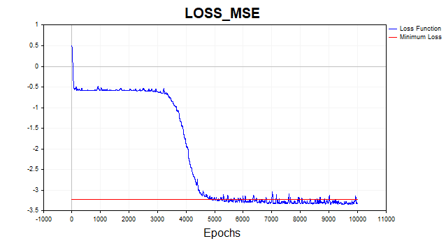
Fig. 6. Loss function in logarithmic scale, SGD

The SGD algorithm (batch_size = 1) converges to the minimum boundary in 4-6 thousand iterations, but let's remember that we are using only one training example out of 81 to update the parameter vector. Therefore, the algorithm on this dataset converges in approximately 50-75 epochs. Not a bad improvement over the previous algorithm, right? I also used momentum here, but since only one data point is used, it doesn't have much of an impact on the convergence speed.

Levenberg-Marquardt algorithm

This good old algorithm is for some reason completely forgotten nowadays, although if your network has up to a couple of hundred parameters, there is simply no equal to it together with L-BFGS.

But there is one important point. The LM algorithm is designed to minimize functions that are sums of squares of other non-linear functions. Therefore, for this method, we will be limited to only a quadratic or root mean square loss function. All things being equal, this loss function does its job perfectly, and there is no big problem here, but we need to know that we will not be able to train the network using this algorithm on other functions.

Let's now take a detailed look at how this algorithm appeared. Let's start with Newton's method:

here

A – inverse Hessian matrix of the F(x) loss function,

g – F(x) loss function gradient,

x – vector of parameters

Now let's look at our quadratic loss function:

here, v is a network error (predicted value minus target), while x is a vector of network parameters that includes all the weights and biases for each layer.

Let's find the gradient of this loss function:

In matrix form, this can be written as:

The key point is the Jacobian matrix:

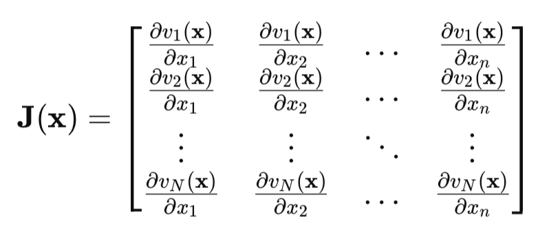
In the Jacobian matrix, each row contains all partial derivatives of the network error with respect to all parameters. Each line corresponds to one example of the training set.

Now let's look at the Hessian matrix. This is the matrix of second partial derivatives of the loss function. Calculating the Hessian is a difficult and expensive task, so an approximation of the Hessian by the Jacobian matrix is used:

If we substitute the Hessian and gradient equations into the Newton's method equation, we obtain the Gauss-Newton method:

But the problem with the Gauss-Newton method is that the [J'J] matrix may not be reversible. To solve this issue, the identity matrix multiplied by the mu*I positive scalar is added to the matrix. In this case, we get the Levenberg-Marquardt algorithm:

The peculiarity of this algorithm is that when the mu parameter takes on large positive values, the algorithm is reduced to the usual gradient descent, which we discussed at the beginning of the article. If the mu parameter tends to zero, we return to the Gauss-Newton method.

Usually training starts with a small mu value. If the loss function value does not become smaller, then the mu parameter is increased (for example, multiplied by 10). Since this brings us closer to the gradient descent method, sooner or later we will achieve a reduction in the loss function. If the loss function has decreased, we decrease the value of the mu parameter by connecting the Gauss-Newton method for faster convergence to the minimum point. This is the main idea of the Levenberg-Marquardt method - to constantly switch between the gradient descent method and the Gauss-Newton method.

The implementation of the backpropagation method for the Levenberg-Marquardt algorithm has its own characteristics. Since the elements of the Jacobian matrix are partial derivatives of the network errors, and not the squares of these errors, the equation for calculating the delta of the last layer of the network, which I gave at the beginning of the article, is simplified. Now delta is simply equal to the derivative of the last layer's activation function. This result is obtained if we find the derivative of the network error (y – target) with respect to y, which is obviously equal to one.

Here is the neural network code itself with detailed comments.

//+------------------------------------------------------------------+
//|                                                           LM.mq5 |
//|                                                           Eugene |
//|                                             https://www.mql5.com |
//+------------------------------------------------------------------+
#property copyright "Eugene"
#property link      "https://www.mql5.com"
#property version   "1.00"
#property script_show_inputs
#include <Graphics\Graphic.mqh>
#include <Math\Stat\Math.mqh>
#include <Math\Stat\Normal.mqh>
enum Plots
  {
   LossFunction_plot,
   mu_plot,
   gradient_plot,
   target_netpredict_plot
  };

matrix weights1,weights2,bias1,bias2;                    // network parameter matrices
matrix n1,n2,act1,act2,new_n1,new_n2,new_act1,new_act2;  // neural layer output matrices
input int    layer1     = 20;                            // neurons Layer 1
input int    Epochs     = 10;                            // Epochs
input double Initial_mu = 0.001;                         // mu
input double Incr_Rate  = 10;                            // increase mu
input double Decr_Rate  = 0.1;                           // decrease mu
input double Min_grad   = 0.000001;                      // min gradient norm
input double Loss_goal  = 0.001;                         // Loss goal
input double sigma_     = 0.1;                           // standard deviation synthetic data
input Plots  plot_      = LossFunction_plot;             // display graph
input bool   plot_log   = false;                         // logarithmic function graph 
input ENUM_ACTIVATION_FUNCTION ac_func      = AF_TANH;   // first layer activation function
input ENUM_ACTIVATION_FUNCTION ac_func_last = AF_LINEAR; // last layer activation function
input ENUM_LOSS_FUNCTION       loss_func    = LOSS_MSE;  // Loss function

double LossPlot[],NetOutput[],mu_Plot[],gradient_Plot[],target_Plot[];
matrix ones_;
double old_error,gradient_NormP2;
double mu_ = Initial_mu;
bool break_forloop = false;
int Sample_,Features;

//+------------------------------------------------------------------+
//| Script start function                                            |
//+------------------------------------------------------------------+
void OnStart()
  {
//--- generate a training sample
   matrix data, target;
   Func(data,target);
   StandartScaler(data);
   Sample_= (int)data.Rows();
   Features = (int)data.Cols();
   ArrayResize(target_Plot,Sample_);
   for(int i=0; i< (int)target.Rows(); i++)
     {
      target_Plot[i] =target[i,0];
     }

   ones_ = matrix::Ones(1,Sample_);
//--- train the model
   ulong start=GetMicrosecondCount();
   Train(data, target, Epochs);
   ulong end = (GetMicrosecondCount()-start)/1000 ;
   Print("Learning time = " + (string)end + " msc");
   int NumberParameters = layer1*(Features+1) + 1*(layer1+1);
   Print("Number Parameters of NN = ",NumberParameters);

//--- generate a test sample
   Func(data,target);
   StandartScaler(data);
//--- test the model
   Test(data,target);
   
//--- display graphs
   PlotGraphic(15,plot_log);
  }
//+------------------------------------------------------------------+
//| Model training method                                            |
//+------------------------------------------------------------------+
bool Train(matrix &data, matrix &target, const int epochs)
  {
//--- create the model
   if(!CreateNet())
      return false;
//--- train the model
   for(int ep = 0; ep < epochs; ep++)
     {
      //--- feed forward
      if(!FeedForward(data))
         return false;
      PrintFormat("Epoch %d, loss %.5f", ep, act2.Loss(target, loss_func));
      //--- arrays for graphs
      ArrayResize(LossPlot,ep+1,10000);
      ArrayResize(mu_Plot,ep+1,10000);
      ArrayResize(gradient_Plot,ep+1,10000);
      LossPlot[ep]       = act2.Loss(target, loss_func);
      mu_Plot [ep]       = mu_;
      gradient_Plot[ep]  = gradient_NormP2;
      //--- Stop training if the target value of the loss function is reached
      if(break_forloop == true){break;}
      //--- backpropagation and update of weight matrix
      if(!Backprop(data, target))
         return false;
     }
//--- Euclidean norm of gradient, mu parameter, RMSE metric
   Print("gradient_normP2 =  ", gradient_NormP2);
   Print(" mu_ = ", mu_);
   double rmse=act2.RegressionMetric(target.Transpose(),REGRESSION_RMSE);
   PrintFormat("rmse %.3f / sigma %.2f ",rmse,sigma_);
//--- array of network output for graph
   ArrayResize(NetOutput,Sample_);
   for(int i=0; i< (int)act2.Transpose().Rows(); i++)
     {
      NetOutput[i]  = act2.Transpose()[i,0];
     }
//--- return result
   return true;
  }
//+------------------------------------------------------------------+
//| Model creation method                                            |
//+------------------------------------------------------------------+
bool CreateNet()
  {
//--- initialize weight matrices
   if(!weights1.Init(layer1,Features) || !weights2.Init(1,layer1))
      return false;
//--- initialize offset matrices
   if(!bias1.Init(layer1,1)  || !bias2.Init(1,1))
      return false;
//--- fill the weight matrices with random values
   weights1.Random(-0.1, 0.1);
   weights2.Random(-0.1, 0.1);
   bias1.Random(-0.1, 0.1);
   bias2.Random(-0.1, 0.1);   
//--- return result
   return true;
  }
//+------------------------------------------------------------------+
//| Feed-forward method                                              |
//+------------------------------------------------------------------+
bool FeedForward(matrix &data)
  {
//--- calculate the first neural layer
//--- n1 pre-activation of the first layer
   n1 = weights1.MatMul(data.Transpose()) + bias1.MatMul(ones_);
//--- calculate the activation function of the act1 first layer
   n1.Activation(act1, ac_func);
//--- calculate the second neural layer
//--- n2 pre-activation of the second layer
   n2 = weights2.MatMul(act1) + bias2.MatMul(ones_);
//--- calculate the activation function of the act2 second layer
   n2.Activation(act2, ac_func_last);
//--- return result
   return true;
  }
//+------------------------------------------------------------------+
//| Backpropagation method                                           |
//+------------------------------------------------------------------+
bool Backprop(matrix &data, matrix &target)
  {
//--- current value of the loss function
   old_error = act2.Loss(target, loss_func);
//--- network error (quadratic loss function)
   matrix loss = act2.Transpose() - target ;
//--- derivative of the activation function of the last layer
   matrix D2;
   n2.Derivative(D2, ac_func_last);
//--- derivative of the first layer activation function
   matrix deriv_act1;
   n1.Derivative(deriv_act1, ac_func);
//--- first layer network error
   matrix D1 = weights2.Transpose().MatMul(D2);
   D1 = deriv_act1 * D1;
//--- first partial derivatives of network errors with respect to the first layer weights
   matrix jac1;
   partjacobian(data.Transpose(),D1,jac1);
//--- first partial derivatives of network errors with respect to the second layer weights
   matrix jac2;
   partjacobian(act1,D2,jac2);
//--- Jacobian
   matrix j1_D1 = Matrixconcatenate(jac1,D1.Transpose(),1);
   matrix j2_D2 = Matrixconcatenate(jac2,D2.Transpose(),1);
   matrix jac   = Matrixconcatenate(j1_D1,j2_D2,1);
// --- Loss function gradient
   matrix je = (jac.Transpose().MatMul(loss));
//--- Euclidean norm of gradient normalized to sample size
   gradient_NormP2 = je.Norm(MATRIX_NORM_FROBENIUS)/Sample_;
   if(gradient_NormP2 < Min_grad)
     {
      Print("Local minimum. The gradient is less than the specified value.");
      break_forloop = true; // stop training
      return true;
     }
//--- Hessian
   matrix Hessian = (jac.Transpose().MatMul(jac));
   matrix I=matrix::Eye(Hessian.Rows(), Hessian.Rows());
//---
   break_forloop = true;
   while(mu_ <= 1e10 && mu_ > 1e-20)
     {
      matrix H_I = (Hessian + mu_*I);
      //--- solution via Solve
      vector v_je = je.Col(0);
      vector Updatelinsolve = -1* H_I.Solve(v_je);
      matrix Update = matrix::Zeros(Hessian.Rows(),1);
      Update.Col(Updatelinsolve,0); // increment of the parameter vector
      
      //--- inefficient calculation of inverse matrix
      //   matrix Update = H_I.Inv();
      //   Update = -1*Update.MatMul(je);
      //---

      //--- save the current parameters
      matrix  Prev_weights1 = weights1;
      matrix  Prev_bias1    = bias1;
      matrix  Prev_weights2 = weights2;
      matrix  Prev_bias2    = bias2;
      //---

      //--- update the parameters
      //--- first layer
      matrix updWeight1 = matrix::Zeros(layer1,Features);
      int count =0;
      for(int j=0; j <Features; j++)
        {
         for(int i=0 ; i <layer1; i++)
           {
            updWeight1[i,j] = Update[count,0];
            count = count+1;
           }
        }

      matrix updbias1 = matrix::Zeros(layer1,1);
      for(int i =0 ; i <layer1; i++)
        {
         updbias1[i,0] = Update[count,0];
         count = count +1;
        }
        
      weights1 = weights1 + updWeight1;
      bias1 = bias1 + updbias1;

      //--- second layer
      matrix updWeight2 = matrix::Zeros(1,layer1);
      for(int i =0 ; i <layer1; i++)
        {
         updWeight2[0,i] = Update[count,0];
         count = count +1;
        }
      matrix updbias2 = matrix::Zeros(1,1);
      updbias2[0,0] = Update[count,0];

      weights2 = weights2 + updWeight2;
      bias2 = bias2 + updbias2;

      //--- calculate the loss function for the new parameters
      new_n1 = weights1.MatMul(data.Transpose()) + bias1.MatMul(ones_);
      new_n1.Activation(new_act1, ac_func);
      new_n2 = weights2.MatMul(new_act1) + bias2.MatMul(ones_);
      new_n2.Activation(new_act2, ac_func_last);
      //--- loss function taking into account new parameters
      double new_error = new_act2.Loss(target, loss_func);
      //--- if the loss function is less than the specified threshold, terminate training
      if(new_error < Loss_goal)
        {
         break_forloop = true;
         Print("Training complete. The desired loss function value achieved");
         return true;
        }
      break_forloop = false;
      //--- correct the mu parameter
      if(new_error >= old_error)
        {
         weights1 = Prev_weights1;
         bias1    = Prev_bias1;
         weights2 = Prev_weights2;
         bias2    =  Prev_bias2;
         mu_ = mu_*Incr_Rate;
        }
      else
        {
         mu_ = mu_*Decr_Rate;
         break; 
        }

     }
//--- return result
   return true;
  }

The algorithm converges if the gradient norm is less than a predetermined number, or if the desired level of the loss function is reached. The algorithm stops if the mu parameter is less than or greater than a predetermined number, or after a predetermined number of epochs have been completed.

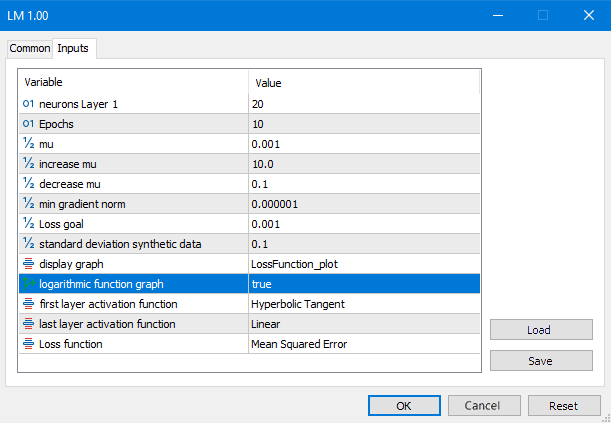
Fig. 7. LM script parameters

Let's look at the result of all this math:

Fig. 8. Loss function in logarithmic scale, LM

It is a completely different picture now. The algorithm reached the minimum boundary in 6 iterations. What if we trained the network on one thousand epochs? We would get a typical overfitting. The picture below demonstrates this well. The network simply starts to memorize Gaussian noise.

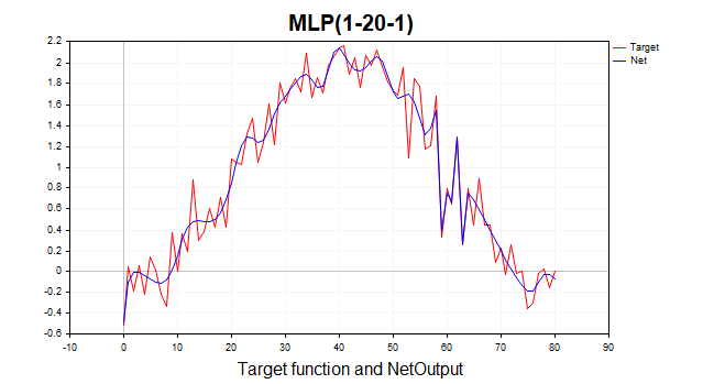
Fig. 9. Typical overfitting, LM, 1000 epochs

Let's look at the metrics on the training and test sets.

Fig. 10. Performance statistics, LM, 1000 epochs

We see RMSE 0.168 with a lower limit of 0.20 and then there is immediate retribution for overfitting on the test of 0.267.

Testing on big data and comparison with Python sklearn library

It is time to test our algorithm on a more realistic example. Now I took two features with 1000 data points. You can download this data along with the LM_BigData script at the end of the article. LM will compete with algorithms from the Python library: SGD, Adam and L-BFGS.

Here is a test script in Python

# Eugene
# https://www.mql5.com

import numpy as np
import time 
import matplotlib.pyplot as plt
import pandas as pd
from sklearn.neural_network import MLPRegressor

# here is your path to the data
df = pd.read_csv(r'C:\Users\Evgeniy\AppData\Local\Programs\Python\Python39\Data.csv',delimiter=';')
X = df.to_numpy()
df1 = pd.read_csv(r'C:\Users\Evgeniy\AppData\Local\Programs\Python\Python39\Target.csv')
y = df1.to_numpy()
y = y.reshape(-1)

start = time.time() 

'''
clf = MLPRegressor(solver='sgd', alpha=0.0, 
                    hidden_layer_sizes=(20),
                    activation='tanh',
                    max_iter=700,batch_size=10,
                    learning_rate_init=0.01,momentum=0.9,
                    shuffle = False,n_iter_no_change = 2000, tol = 0.000001)
'''

'''
clf = MLPRegressor(solver='adam', alpha=0.0, 
                    hidden_layer_sizes=(20),
                    activation='tanh',
                    max_iter=3000,batch_size=100,                                    
                    learning_rate_init=0.01,
                    n_iter_no_change = 2000, tol = 0.000001)
'''

#'''
clf = MLPRegressor(solver='lbfgs', alpha=0.0, 
                    hidden_layer_sizes=(100),
                    activation='tanh',max_iter=300,
                    tol = 0.000001)
#'''                    
                       
clf.fit(X, y)
end = time.time() - start          # training time

print("learning time  =",end*1000) 
print("solver = ",clf.solver);      
print("loss = ",clf.loss_*2)
print("iter = ",clf.n_iter_)
#print("n_layers_ = ",clf.n_layers_)
#print("n_outputs_ = ",clf.n_outputs_)
#print("out_activation_ = ",clf.out_activation_)

coef = clf.coefs_
#print("coefs_ = ",coef)
inter = clf.intercepts_  
#print("intercepts_ = ",inter) 
plt.plot(np.log(pd.DataFrame(clf.loss_curve_)))
plt.title(clf.solver)
plt.xlabel('Epochs')
plt.ylabel('Loss')
plt.show()  

To compare the algorithms correctly, I multiplied the loss function in Python by 2, since in this library it is calculated like this:

return ((y_true - y_pred) ** 2).mean() / 2

In other words, the developers additionally divided MSE into 2. Below are typical results from optimizers. I tried to find the best hyperparameter settings for these algorithms. Unfortunately, this library does not provide the ability to initialize the values of the starting parameters so that all algorithms start from the same point in the parametric space. There is also no way to set a target threshold for the loss function. For LM the loss function target is set to 0.01, for Python algorithms I tried to set the number of iterations that approximately achieves the same level.

Test results of MLP with one hidden layer, 20 neurons:

1) Stochastic gradient descent  

• loss mse – 0,00278
• training time  - 11459 msc

Fig. 11. SGD, 20 neurons, loss = 0.00278

2) Adam          

•  loss mse – 0.03363
•  training time  - 8581 msc

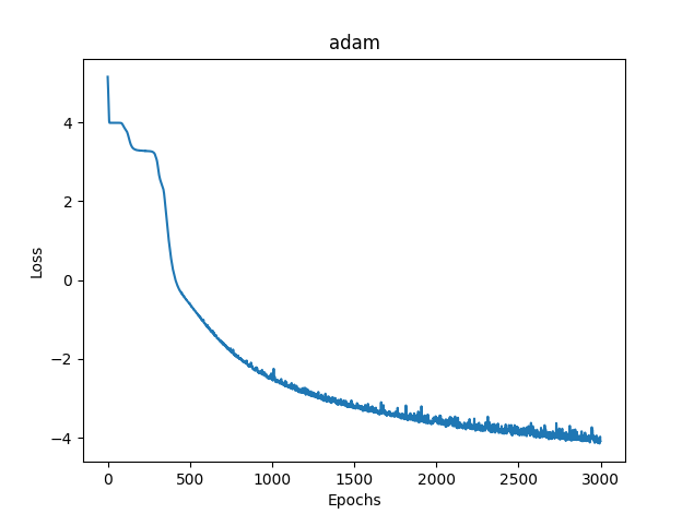
Fig. 12. Adam, 20 neurons, loss = 0.03363

3)L-BFGS

• loss mse – 0.02770
• training time - 277 msc

Unfortunately, it is not possible to display the loss function graph for L-BFGS.

4) LM MQL5

•  loss – 0.00846
•  training time — 117 msc

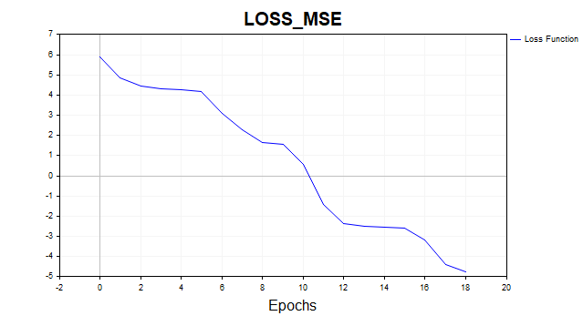
Fig. 13. LM, 20 neurons, loss = 0.00846

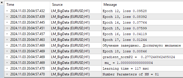
As for me, the algorithm easily competes with L-BFGS and can even give it a head start. But nothing is perfect. As the number of parameters increases, the Levenberg-Marquardt method begins to lose to L-BFGS.

100 neurons L-BFGS:

• loss mse – 0.00847
• training time - 671 msc

100 neurons LM:

• loss mse – 0.00206
• training time  -  1253 msc

100 neurons correspond to 401 network parameters. It is up to you to decide whether this is a lot or a little, but in my humble opinion, this is excess power. In cases up to 100 neurons, LM clearly has an advantage.

Conclusion

In this article, we discussed and implemented the basic and simplest neural network training algorithms:

• gradient descent
• gradient descent with momentum
• stochastic gradient descent

At the same time, we briefly touched on the issues of convergence and retraining of neural networks.

But most importantly, we built a very fast Levenberg-Marquardt algorithm that is ideal for online training of small networks.

We compared the performance of neural network training algorithms used in the scikit-learn machine learning library, and our algorithm turned out to be the fastest when the number of neural network parameters does not exceed 400 or 100 neurons in the hidden layer. Further, as the number of neurons increases, L-BFGS begins to dominate.

For each algorithm, separate scripts have been created, with detailed comments:

#	Name	Type	Description
1	SD.mq5	Script	Gradient descent
2	Momentum_SD.mq5	Script	Gradient descent with momentum
3	SGD.mq5	Script	Stochastic gradient descent
4	LM.mq5	Script	Levenberg-Marquardt algorithm
5	LM_BigData.mq5	Script	LM algorithm, test on two-dimensional features
6	SklearnMLP.py	Script	Python algorithms test script
7	FileCSV.mqh	Include	Reading text files with data
8	Data.csv, Target.csv	Csv	Python script features and purpose
9	X1.txt, X2.txt, Target.txt	Txt	LM_BigData.mq5 script features and purpose