Gaussian Processes in Machine Learning: Regression Model in MQL5

Introduction

Gaussian processes (GPs) are a Bayesian non-parametric modeling framework widely used in machine learning for regression and classification problems. Unlike many traditional models that provide only point forecasts, GPs generate a full probability distribution for the predictive values. This allows the model to provide not only point predictions but also uncertainty estimates, typically expressed as confidence intervals. This is a distinctive feature of the Bayesian approach, which combines prior knowledge with observed data to obtain a predictive distribution.

GPs belong to the class of kernel methods that use covariance functions (or kernels) to model dependencies between data. The ability to combine different kernels (e.g. by addition or multiplication) allows for a certain flexibility in describing possible predictive functions. Each kernel has its own hyperparameters that need to be optimized to achieve maximum model accuracy.

In this article, we will examine in detail the forecasting process using a Gaussian process regression model, clearly demonstrating how GPs allow not only to generate accurate forecasts but also to comprehensively assess their uncertainty.

What is a Gaussian process?

From a probabilistic perspective, a Gaussian process is a random process that describes a probability distribution over functions. Unlike the ordinary normal distribution, which describes a single random variable, the GP defines a collection of random variables, any finite subset of which obeys the multivariate normal distribution.

In machine learning, GPs refer to non-parametric models that do not require a pre-defined function form (e.g., linear or polynomial, as in classical regression). Instead, the GP models a latent function f(x) that is assumed to capture the true dependencies in the data. However, the function f(x) itself is not directly observable; we only have access to its values with noise at given x points. The GP model is based on the assumption that the distribution of this unknown f(x) function is normal:

f (x)~ N( μ, Σ),

where:

• f(x) — hidden (latent) function whose values at the observed points we want to simulate,
•  μ — vector of mean values depending on the prior mean function (often taken to be zero for simplicity),
•  Σ — covariance matrix whose elements are determined by the covariance function (or kernel) K(x, x'), which specifies the degree of correlation between points x and x'.

The key idea of GP is to model the distribution of functions through a covariance structure defined by a kernel, which in turn determines various properties of the functions, such as their smoothness, periodicity, non-stationarity, etc.

The main goal of GP is to reconstruct the latent function f(x) based on a finite data set D=(X,y), where X is a set of features and y are noisy observations.

Bayesian approach to GP

Gaussian processes use a Bayesian approach to statistical inference that combines prior knowledge with observed data to make probabilistic predictions. This distinguishes GP from many other machine learning methods (such as neural networks or SVMs) by allowing it to not only predict values but also estimate their uncertainty. This approach is based on Bayes' theorem:

where:

• P(H) — prior probability: the initial probability of the H hypothesis, reflecting prior knowledge or assumptions before observing the data,
• P(D|H) — likelihood: the probability of observing the data D given hypothesis H,
• P(H|D) — posterior probability: the probability of H hypothesis after observing D data,
• P(D) — marginal probability of the data (normalizing constant) that ensures the correctness of the posterior distribution.

In the context of GP, the Bayesian approach is applied as follows. H hypothesis is interpreted as a distribution over functions f(x), from which our data sample could be generated, and D data is the training dataset (X, y).

In the GP setting, Bayes’ theorem takes the following form:

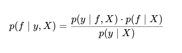
where:

• p(f |X) — prior distribution over f functions,
• p(y |f, X) — likelihood,
• p(f |y, X) — posterior distribution over f functions,
• p(y |X) — marginal likelihood (evidence). Used to optimize Gaussian process hyperparameters.

In GP, since both the prior and likelihood functions are Gaussian, the posterior distribution is also a Gaussian process, but with updated mean and covariance functions that incorporate information learned from the data. This is due to the mathematical property of conjugacy of Gaussian distributions, which makes deriving the equation for predictions relatively simple.

Prior distribution

The prior distribution describes our initial guesses about possible functions before we see the data. Essentially, the prior is a set of possible functions, from which the GP will select the most appropriate ones based on the training data. The kernel plays a key role in defining the properties of these functions. There are many types of kernels, each suitable for different types of data, for example:

RBF (Gaussian kernel) models smooth non-linear functions:

where:

• σ_f  — amplitude, specifies the scale of variations (in the params.rbf.sigma_f code),
• l — length scale controls the decay rate of the correlation (params.rbf.length),
• ∥x−x′∥ — Euclidean distance between points x and x'.

Linear kernel models linear dependencies:

• x*x' — scalar product of two vectors,
• σ_l — linear trend scale (params.linear.sigma_l)

Periodic kernel captures cyclical patterns:

• σ_f  — amplitude, sets the scale of oscillations (params.periodic.sigma_f),
• l — scale length, controls the smoothness of oscillations (params.periodic.length),
• p — period determines the repetition frequency (params.periodic.period).

To visualize the prior distribution, consider samples of f(x) functions generated using different kernels. Figure 1 shows samples from a prior distribution with an RBF kernel. The trajectories are smooth non-linear functions that vary depending on the kernel parameters.

Fig. 1 Samples of f functions f from the prior GP distribution (RBF kernel)

Figure 2 shows samples from a prior distribution with a linear kernel. The trajectories are straight lines with varying slopes, reflecting the kernel's ability to model linear trends.

Fig. 2. Samples of f functions from the prior distribution of the GP (linear kernel)

Fig. 3 shows samples with a periodic kernel. The trajectories are cyclic functions with p period, making the kernel ideal for modeling periodic components.

Fig. 3. Samples of f functions from the prior distribution of the GP (periodic kernel)

Figure 4 shows the trajectories of the well-known Wiener process with the K(x,x') = min(x, x') covariance function. 

Fig. 4. Samples of f functions from the prior distribution of the GP with the covariance function of the Wiener process

The flexibility of the GP is achieved through the ability to combine kernels (by adding or multiplying them), which allows modeling functions with a variety of properties, such as a combination of linear and non-linear trends, periodic oscillations, etc. Samples were generated using the SamplesPrior script.

Likelihood

In Gaussian processes, the p(y |f, X) likelihood describes the probability of observing y data given a particular f function from the prior distribution and X data. It plays a key role in Bayesian inference by relating the prior distribution over functions to the observed data. For a data set, the likelihood is set by the multivariate normal distribution:

where:

• f(x) — vector of values of the hidden function at X points,
• σy^2 — noise variance,
• ∥y−f(x)∥^2 — square of the Euclidean norm of the difference between the observed data and the values of the f function.

The equation shows that the likelihood is higher the closer the values of the f function are to the observed y data.

Posterior distribution

The posterior distribution is the result of a Bayesian update of the prior distribution given the observed data and the likelihood. It describes the distribution of the latent function values f(x) at new test points X*. This distribution is characterized by the μ* updated mean representing the forecast and the Σ* covariance matrix describing the uncertainty of the forecasts.

Thus, the prior distribution specifies a set of functions, the likelihood "weights" them based on the data, and the posterior distribution provides the most likely function with an estimate of the uncertainty.

GP regression with Gaussian likelihood

Gaussian processes, in combination with Gaussian observation noise, allow the regression problem to be solved in analytical form using linear algebra methods. This significantly simplifies calculations and eliminates the need to use complex numerical methods. GPs are suitable for modeling both noisy and noise-free data. Let's first consider the idealized case where the y target values are the noise-free true values of the function, that is, when y = f(x) (interpolation scenario).

Non-noisy case: Interpolation 

Suppose we have a data set of D = {(xn, yn) : n = 1 : N}, where yn = f(xn) is the exact noise-free observation of the f function evaluated at the xn point. Our task is to predict the values of the f* function for the X* test set of N*×d size.

For X training points and X* test points, the joint prior distribution of the f and f* function values is a multivariate normal distribution:

where:

• f — vector of true values of the hidden function at training points,
• f* — vector of true values of the hidden function at test points,
• m(X) — vector of mean values of the function for training points (vector of zeros for simplicity),
• m(X*) — vector of mean values of the function for test points (vector of zeros for simplification),
• K(X,X) — NxN covariance matrix between all pairs of training points,
• K(X,X*) — NxN* covariance matrix between training and test points,
• K(X*,X*) — N*xN* covariance matrix between all pairs of test points
• N — number of input data points,
• N* — number of test data points,
• d — dimension of the input data (number of features).

Since the y observations in this case exactly correspond to f (y=f), that is, the likelihood is a delta function, we can immediately go to the conditional distribution of f* given y. Due to the properties of the conditional distributions of the multivariate normal distribution, the posterior distribution for f* given the y observed data is:

where:

• μf* — posterior mean, the best prediction of the values of the f* hidden function at new (test) points based on the training data,
• Σf* — posterior covariance matrix for the test points. It quantifies the uncertainty in the prediction of the f* hidden function.

Noise case: Regression

In real-world problems, y data usually contain unpredictable noise: y=f(X)+ϵ, where ϵ∼N(0,σ^2) is Gaussian noise. In this case, the GP does not interpolate the training data exactly (i.e., it does not pass exactly through each point), but instead smooths it, taking into account the expected level of noise. The posterior distribution for noisy data is modified by adding the noise variance to the diagonal elements of the covariance matrix of the training data:

The noise parameter of σ​ is a hyperparameter of the model and is optimized together with the kernel parameters. 

A very important point: by adding noise, we gain the ability to predict confidence intervals not only for the latent function of f*, but also for new y* observations. Unlike the noise-free case, where the predictive distributions for f* and y* were the same, these distributions now differ. The main difference lies in their covariance matrices. The Σf* covariance reflects the uncertainty of the latent function itself at the test points. The Σy* covariance includes the uncertainty of the latent function plus the variance of the observation noise.

• μy* — posterior mean for the new y* observation. It coincides with μf* since the expected value of the noise is zero,
• Σy* — posterior covariance for the new y* observation.  

Therefore, if we are interested in confidence intervals for new y* observations, rather than for new values of the f* latent function, we should use this equation.

To visualize how Gaussian processes adapt to data, consider a visualization of samples of f functions generated from the posterior distribution in the absence of noise. Figure 5 shows three f functions constructed after observing five training points using the RBF kernel.

Fig. 5. Samples of f functions from the posterior distribution (RBF kernel, without noise)

Before any data is observed, the prior distribution given by the GP describes an infinite set of functions. After we add training data, the posterior distribution restricts this set, leaving only functions that exactly pass through the observed points. In other words, it focuses exclusively on those functions that accurately interpolate the data. 

At the X training points, the variance (the diagonal elements of the posterior covariance matrix Σ*) is zero, meaning there is no uncertainty at these points: all functions sampled from the posterior distribution are guaranteed to pass exactly through the training points. Outside of training points, functions may vary, reflecting model uncertainty in areas where data is missing. However, their behavior is still determined by the structure of the chosen kernel, in this case RBF.

Now consider a graph of samples of f functions from the posterior distribution when the observed y data contain Gaussian noise. (Fig. 6)

Fig. 6. Samples of f functions from the posterior distribution (RBF kernel, with noise)

In the presence of noise, the posterior functions do not need to exactly pass through the observed y data. This means that the set of possible functions that can explain the data becomes wider, as they can deviate from the observed values within the noise. The gray dashed lines represent 2-sigma confidence intervals covering about 95% of the probability of the f* posterior distribution. In regions far from the training data, the uncertainty increases even more and the confidence intervals become significantly wider, indicating a decrease in the model's confidence in these regions. It is important to note that the gray dashed lines represent confidence intervals for the f* latent function, not for new y* observations. 

Gaussian process hyperparameter optimization

The performance of a Gaussian process model depends heavily on the optimal choice of its hyperparameters, which allows the model to fit the data, maximizing its ability to explain the observed relationships. Such hyperparameters include kernel parameters and noise variance. In GP, optimization is performed using negative log marginal likelihood (NLML) minimization:

Direct calculation of (K+σ^2*I)^−1 * y is computationally expensive for large n, since it requires inverting the n×n matrix. Therefore, Cholesky decomposition is used to make the computation more efficient and robust. Taking this decomposition into account, the NLML equation can be rewritten as:

• z — vector obtained by solving a system of linear equations using the Cholesky decomposition,    z=L^−1*y
• L — the lower triangular matrix from the Cholesky decomposition K+σ^2*I = LL^T

This equation is implemented in the NegativeLogMarginalLikelihood function.

//+------------------------------------------------------------------+
//| Calculate the negative log-likelihood                            |
//+------------------------------------------------------------------+
double NegativeLogMarginalLikelihood(const matrix &x, const matrix &y, int &kernel_list[], KernelParams &params)
{
   int n = (int)x.Rows();

   //--- Calculate the K covariance matrix
   matrix K = ComputeKernelMatrix(x, x, kernel_list, params);
   
   //--- Add white noise variance if KERNEL_WHITE is selected
    double white_noise_variance = 0.0;
    for (int i = 0; i < ArraySize(kernel_list); i++)
    {
        if (kernel_list[i] == KERNEL_WHITE)
        {
            white_noise_variance = params.white.sigma * params.white.sigma;
            break; 
        }
    }
   // Adding a little jitter prevents problems,
   // if the K matrix is singular or close to singular  
   // due to the peculiarities of the calculations or the chosen kernel
    double jitter = 1e-6;
    K += matrix::Identity(n, n) * (white_noise_variance + jitter);
     
   // ---Perform the Cholesky decomposition: K + sigma^2*I = L * L^T
   matrix L;
   if (!K.Cholesky(L))
   {
      Print("Error: Cholesky decomposition failed");
      return DBL_MAX;
   }

  //--- Solve the linear system L * z = y to find  z = L^(-1) * y
   vector z = L.LstSq(y.Col(0));
   if (z.Size() == 0)
   {
      Print("Error: Unable to solve the system L * z = y");
      return DBL_MAX;
   }

   //--- Calculate the first term in the NLML equation: 
   // 1/2 * y^T * (K + sigma^2*I)^-1 * y = 1/2 * z^T * z
    double data_term = 0.5 * z @ z; // Scalar product z^T * z   

   //--- Calculate the second term: 1/2 * log|K + sigma^2*I| = sum(log(L_ii))
   vector diag = L.Diag();
   double log_det = 0.0;
   for (int i = 0; i < n; i++)
      log_det += MathLog(diag[i]); // sum the logarithms of the L diagonal elements
  
   //--- Calculate the third term: n/2 * log(2π)
   double const_term = 0.5 * n * MathLog(2 * M_PI);

   return data_term + log_det + const_term;
   
}

The K covariance matrix is calculated using the ComputeKernelMatrix function, which sums the contributions from all selected kernels (e.g. RBF, Linear, Periodic, etc.).

//+------------------------------------------------------------------+
//| Calculate the covariance matrix                                  |
//+------------------------------------------------------------------+
matrix ComputeKernelMatrix(const matrix &X1, const matrix &X2, int &kernel_list[], KernelParams &params)
{
   matrix K  = matrix::Zeros(X1.Rows(), X2.Rows());
   for (int i = 0; i < ArraySize(kernel_list); i++)
   {
      switch (kernel_list[i])
      {
         case KERNEL_RBF:
            K += RBF_kernel(X1, X2, params.rbf.sigma_f, params.rbf.length);
            break;
         case KERNEL_LINEAR:
            K += Linear_kernel(X1, X2, params.linear.sigma_l);
            break;
         case KERNEL_PERIODIC:
            K += Periodic_kernel(X1, X2, params.periodic.sigma_f, params.periodic.length, params.periodic.period);
            break;
         case KERNEL_WHITE:
            // WhiteKernel is added separately as sigma^2 * I
            break;
      }
   }
   return K;
}

NLML is used as the objective function for hyperparameter optimization in the OptimizeGP function. Optimization is performed using the BLEIC method from the ALGLIB library. 

//+------------------------------------------------------------------+
//| Gaussian process hyperparameter optimization                     |
//+------------------------------------------------------------------+
KernelParams OptimizeGP(int &kernel_list[], matrix &x_train, matrix &y_train)
{
   double w[]; // Array of initial hyperparameter values 
   double s[]; // Array of scales for hyperparameters used for normalization in optimization
   double bndl[], bndu[]; // Arrays of lower and upper bounds for each hyperparameter    
   CObject Obj;
   CNDimensional_GP ffunc(kernel_list, x_train, y_train);// Object of a class implementing the NLML target function
   CNDimensional_Rep frep; // Object for storing the optimization report 
   
   // Initialize parameters
   InitializeKernelParams(kernel_list, w, s, bndl, bndu);
   /*
   The total number of parameters (num_params) is calculated depending on the kernel types in kernel_list.
   The initial values of the w parameters, scale and bounds for the parameters are set  
   */

   CMinBLEICStateShell state;
   CMinBLEICReportShell rep; // Object for storing optimization results.

   double epsg = 0;  // Gradient precision (0 means gradient stopping is disabled)
   double epsf = 0.0001; // Precision by function value 
   double epsw = 0; // accuracy by parameters 
   double diffstep = 0.0001; // Step for numerical calculation of derivatives.
   double epso = 0.00001; // Parameters for external and internal convergence conditions in BLEIC
   double epsi = 0.00001;

   CAlglib::MinBLEICCreateF(w, diffstep, state); // Create a BLEIC optimization object with w initial parameters and diffstep for numerical derivatives
   CAlglib::MinBLEICSetBC(state, bndl, bndu); // Set parameter bounds (bndl, bndu).
   CAlglib::MinBLEICSetScale(state, s); // Sets the scale of (s) parameters.
   CAlglib::MinBLEICSetInnerCond(state, epsg, epsf, epsw); 
   CAlglib::MinBLEICSetOuterCond(state, epso, epsi);
   CAlglib::MinBLEICOptimize(state, ffunc, frep, 0, Obj);
   CAlglib::MinBLEICResults(state, w, rep);
   Print("TerminationType =", rep.GetTerminationType()); // Optimization completion code
   /*
                * -8    internal integrity control  detected  infinite or
                        NAN   values   in   function/gradient.   Abnormal
                        termination signalled.
                * -3   inconsistent constraints. Feasible point is
                       either nonexistent or too hard to find. Try to
                       restart optimizer with better initial approximation
                *  1   relative function improvement is no more than EpsF.
                *  2   scaled step is no more than EpsX.
                *  4   scaled gradient norm is no more than EpsG.
                *  5   MaxIts steps was taken
                *  8   terminated by user who called minbleicrequesttermination().
                       X contains point which was "current accepted"  when
                       termination request was submitted.   
   */
   Print("IterationsCount =", rep.GetInnerIterationsCount()); // Number of iterations

   Print("Parameters:");
   PrintKernelParams(w, kernel_list); // Display optimized parameters in the log
   Print("NLML = ", ffunc.GetNLML()); // final NLML value for optimal parameters

   KernelParams optimized_params;    
   CRowDouble parameters = w;   
   // determine the correct distribution of parameters across kernels 
   ExtractKernelParams(parameters, kernel_list, optimized_params); 

   return optimized_params;
}

GP regression in MQL5

To illustrate the capabilities of the Gaussian process regression model, let us consider an example using synthetic data. The implementation is presented in the GP_Regressor script, which demonstrates creating, training and testing the model.

Data generation is performed using the Dataset function, which produces matrices of synthetic data for training and testing. The dataset consists of 100 points uniformly distributed in the range [−5,5] and represents the function of y=sin⁡(x)+0.5x with added Gaussian noise. This approach allows simulating real data containing both a linear trend and a periodic component, taking into account uncertainty.

To build a regression model, it is necessary to determine the list of kernels that form the covariance function. Each kernel makes a unique contribution to the K covariance matrix, determining the nature of the dependencies the model is able to capture. The kernel list is configured using the SetKernelList function, which generates the kernel_list array based on the kernel_combination input parameter (enum type KernelCombination). The following combinations are supported:

• COMBINATION_1: [RBF, Linear, White] (3 kernels),
• COMBINATION_2: [RBF, Linear, Periodic, White] (4 kernels),
• COMBINATION_3: [RBF, White] (2 kernels).

The flexibility of choosing a combination of kernels allows the model to be adapted to various types of data, be it linear trends, periodic fluctuations, or complex non-linear dependencies.
After selecting the kernels, the model hyperparameters are optimized using the OptimizeGP function. This function minimizes the negative log-likelihood (NLML) by returning the KernelParams structure containing the optimal parameters for each kernel, such as amplitude (σ_f), scale length (l) or period (p).

Once the optimal parameters have been found, we move on to the forecast using the Predict function.

//+------------------------------------------------------------------------+
//| Predict the Gaussian posterior distribution for new points             |    
//+------------------------------------------------------------------------+
GPPredictionResult Predict(const matrix &x_train, const matrix &y_train, const matrix &x_test, 
             int &kernel_list[], KernelParams &params)
{
  GPPredictionResult result; 

   //  Calculate the K covariance matrix for the training points 
   matrix K = ComputeKernelMatrix(x_train, x_train, kernel_list, params); 
   // Obtain the observation noise variance
    double observation_noise_variance = 0.0;
    for (int i = 0; i < ArraySize(kernel_list); i++)
    {
        if (kernel_list[i] == KERNEL_WHITE)
        {
            observation_noise_variance = params.white.sigma * params.white.sigma;
            break;
        }
    }
   
   // Form a noise matrix for the training data: K + sigma_n^2 * I
   matrix K_noisy_train = K + matrix::Identity((int)x_train.Rows(), (int)x_train.Rows()) * observation_noise_variance;  
   // Calculate the K* cross-covariance matrix between training and test points   
   matrix K_star = ComputeKernelMatrix(x_train, x_test, kernel_list, params);
   // Calculate the posterior mean
   matrix inv_term = K_noisy_train.Inv(); 
   result.mu_f_star = K_star.Transpose() @ (inv_term @ y_train); // Matches mu_y_star
     
   // Calculate the posterior covariance matrix for the latent function (Sigma_f_star)
    matrix K_star_star = ComputeKernelMatrix(x_test, x_test, kernel_list, params);
    result.Sigma_f_star = K_star_star - K_star.Transpose() @ (inv_term @ K_star);
    
   // Calculate the posterior covariance matrix for a new observation (Sigma_y_star)
   // Sigma_y_star = Sigma_f_star + sigma_n^2 * I
    result.Sigma_y_star = result.Sigma_f_star + matrix::Identity((int)x_test.Rows(), (int)x_test.Rows()) * observation_noise_variance;

    return result;
   
}

The Predict function is a key element of the GP model implementation, as it does not simply return the predicted values, but provides full information about the posterior distribution at the test points. The function returns the GPPredictionResult structure that contains:

• posterior mean for the f* latent function (μf* = μy*),
• Σf* posterior covariance matrix for the f* latent function,
• Σy* posterior covariance matrix for the y* values. The matrix includes both the uncertainty of the latent function and the variance of the observation noise (σ^2) determined during the optimization of the WhiteKernel parameter.

Now let's look at the forecast results for different combinations of kernels. To begin, let's try to predict our function using only the RBF kernel, assuming that there is noise in the data (Fig. 7).

Fig. 7. Forecast using RBF kernel

• Red dots — training data (TrainData),
• Blue line — predicted mean,
• Green stars — forecast for test points (X*),
• Blue dots - test data outside the training range,
• Gray dashed lines — confidence intervals (± 2 sigma for f* or y*)

Here we see that as the test points move away from the training data range [-5,5], the predictions tend to the GP prior mean, which is usually taken to be zero. This happens because away from the training data, the K* covariances (between x* new points and x training points) for the RBF kernel decrease exponentially to zero. Therefore, the RBF kernel is better suited for data interpolation, but its use for extrapolation is limited due to the rapid decay of correlations.

 To improve extrapolation, add a linear kernel (Fig. 8).

Fig. 8. Forecast using the sum of RBF and linear kernel, f* intervals

The linear kernel models linear relationships, making it suitable for extrapolation, especially if the data has a linear or nearly linear trend, as in our example with the y=sin⁡(x)+0.5x function. Including a linear kernel improved forecasts outside the training data range by capturing a linear component (0.5x). However, as can be seen from the graph, the model still does not fully reflect the structure of the data, missing its periodic component.

A periodic kernel is used (Figure 9) to model seasonal or cyclical variations, such as sin⁡(x) in our data.

Fig. 9. Forecast using the sum of RBF, periodic and linear kernels, f* intervals

After adding the periodic kernel, the model achieved a near-perfect prediction because it was able to capture all the significant dependencies present in the data. As a result, the confidence intervals for f* (the latent function) practically merge with the posterior mean. For observed y* values, on the contrary, the confidence intervals are much wider, which is logical since they take into account the variance of the observation noise, as shown in Fig. 10.

Fig. 10. Forecast using the sum of RBF, periodic and linear kernels, y* intervals

An important note about forecasts in GP. Without proper consideration of noise variance, confidence intervals for f*(x) can be mistakenly interpreted as forecast intervals for y*. To obtain correct forecast intervals for y*, it is necessary to explicitly include the noise variance in the covariance matrix, which is implemented in the Predict function.

Conclusion

In this article, we took a detailed look at the basics of Gaussian processes using a regression problem as an example. We studied the key components of the GP: the prior distribution, the likelihood, and the posterior distribution, which provides full probabilistic forecasts with quantified uncertainty. We have implemented the basic kernel functions, such as RBF, Linear and Periodic, although there are of course many more.

Particular attention was paid to hyperparameter optimization, which is critical for adapting the GP to specific data. We demonstrated that this optimization is achieved by minimizing the negative log-marginal likelihood (NLML), where Cholesky decomposition is used to improve computational efficiency and numerical stability. The gradient method BLEIC from the ALGLIB library was used as an optimizer in the implemented model.

This article focuses on the basic principles of GP, and a number of advanced topics are left out of it. These include, for example, the use of analytic expressions for NLML gradients, which can significantly improve optimization efficiency, as well as the use of sparse approximations, which are critical for processing large amounts of data. These directions open up prospects for further GP model research.

#	Name	Type	Description
1	GP_Samples_Prior.mq5	Script	Demonstration of samples from the prior distribution
2	GP_Samples_Posterior.mq5	Script	Demonstration of samples from the posterior distribution
3	GP_Regressor	Script	Building a regression model