Self Optimizing Expert Advisors in MQL5 (Part 14): Viewing Data Transformations as Tuning Parameters of Our Feedback Controller

Preprocessing is a powerful and yet often overlooked tuning parameter in any machine learning framework or pipeline.

It is an important control knob in the pipeline that is often hidden away in the shadows of its bigger brothers. Commonly, optimizers or shiny model architectures mainly get the focus and research work, and large amounts of academia are poured into those directions. But little time is spent studying the effects of pre-processing techniques.

Silently, the pre-processing that we apply to the data at hand impacts model performance in ways that can be surprisingly large. Even small percentage improvements made in pre-processing can compound over time and materially affect the profitability and risk of our trading applications.

All too often, we rush through the activity of preprocessing without giving much thought or much time to validating whether we have truly identified the best transformation possible for the input data.

The advanced optimizers and machine learning architectures that we depend on in our modern age are quietly being held back—or empowered—by the transformations that we apply to the data at hand. Unfortunately, at the time of writing, there is no established framework to prove that any given transformation is optimal. Not only that, but we also have no measure of confidence that no better alternative transformation exists. In fact, little research explores combining different transformations into hybrid solutions—and it is here where untapped performance could potentially be unlocked.

Therefore, our objective is to improve the efficiency of a feedback controller that we carefully built together in a previous discussion (link provided here).

Beyond ordinary profitability, we aim to observe reductions in risk, and more robust—and to a certain extent more mature—trading behavior being demonstrated by our trading application. In essence, this exercise treats preprocessing itself as a tuning parameter in its own right—one that can materially shift outcomes of trading applications if handled correctly.

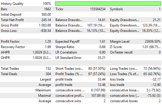
Figure 1: The old backtest statistics setup by the old version of our feedback controlle

The performance of our old feedback controller was surely acceptable by all measures; however, needless to say, we will demonstrate that spending time testing for the right transformations can potentially unlock alpha in your strategy that was dormant because the signal was not effectively exposed. 

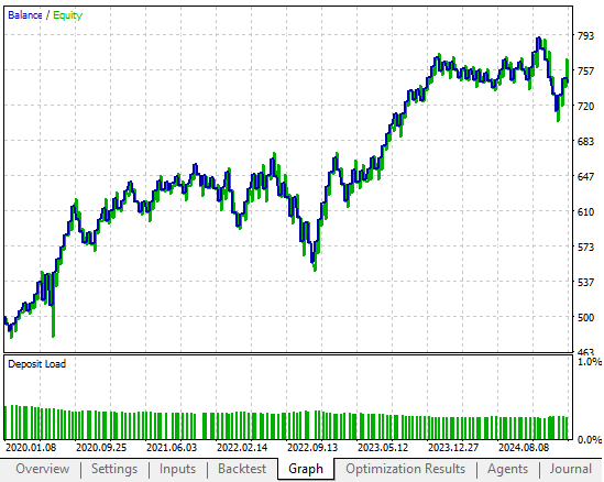
Figure 2: The old equity curve we are aiming to outperform by identifying an appropriate transformation to apply to our input data

Failure to expose the rich patterns in your dataset, erodes investor capital over time. We tested three distinct transformations on the input data that we fed to our feedback controller. To have a control setup, we ran a benchmark with raw and untransformed inputs from our previous discussion. Subsequently, each transformation we evaluated was tested over identical historical data while holding all other variables constant. Performance was measured in terms of profitability, Sharpe ratio, the number of trades placed, the total gross loss accrued, and the total proportion of profitable trades. This allowed us to isolate the effects of pre-processing while maintaining a fair comparison across all three tests.

The first transformation we tested was the standard statistical z-score. The z-score is calculated by subtracting the mean of each column and dividing each column by its standard deviation. We observed that this transformation reduced our profitability levels by 30 percent from the baseline. This is not attractive by any measure. Additionally, it dropped our Sharpe ratio by a staggering 10 percent from the baseline performance level.

Therefore, the z-score transformation was not ideal for us. Afterward, we applied a transformation borrowed from the field of linear algebra. This transformation is known as unit scaling, and it is performed by dividing a matrix by its norm. In this particular case, we chose the L1 norm of the matrix to be the divisor. After scaling with the L1 norm, we noticed that our application’s profitability levels improved by 12 percent over the baseline, which is attractive. In addition to that, the Sharpe ratio improved by 30 percent off the unit scaling.

Another great sign of trading skill is when our application can reach higher levels of profitability with fewer trades in total. This was the case again: after unit scaling, the total number of trades required declined by 8 percent, and the total loss accrued also declined by 15 percent. Lastly, the total proportion of winning trades increased by 5 percent. Therefore, this gave us strong confidence that unit scaling had positively improved the performance of our feedback controller.

Lastly, we tested a hybrid of z-score and unit scaling. Unfortunately, this destroyed all the improvements we gained from unit scaling alone. Our profitability fell by 58 percent below the baseline, and our Sharpe ratio declined by 19 percent. Therefore, despite our strong intuition, combining these two transformations into a hybrid was destructive for performance and did not expose any additional structure that we could learn from.

Therefore, from all of this, we can easily discern that preprocessing is not just another means to an end when building machine learning models for trading. Rather, pre-processing is, in itself, its own strategy. The choice of transformation silently colors the performance of our machine learning models—shaping profits, distorting losses, and inadvertently changing our risk exposure in ways we do not directly understand.

Classical statistical learning offers little, if any, guidance in this direction. There are no universal, agreed standards beyond brute-force exploration through cross-validation for partitions. This means investing time in benchmarking pre-processing pipelines and treating them for what they are: high-leverage tuning parameters in our machine learning pipeline.

This should also incentivize other researchers and article writers to explore more and more transformations that could be applied in our domain. Because in domains such as image identification and speech recognition, machine learning practitioners often employ robust and extensive pipelines of transformations alone before any prediction is even attempted. And yet in fields such as ours, in financial machine learning, we often spend very little time building robust pipelines of pre-processing transformations.

Under the current conditions we face, brute-force testing is a sound strategy. The more we explore, the better we understand the characteristics of each transformation we apply to this particular market. This helps us map which transformation could be best among all the transformations we have observed.

Reviewing The Current Baseline

Before we get started, it is important to first review the control setup that we want to outperform. Any optimization exercise is difficult to interpret without a benchmark or baseline performance level to compare against. Therefore, we will begin by quickly reviewing the initial feedback controller we implemented. For returning readers, the following code will already be familiar. For first-time readers, I will highlight the key takeaways from the application we built and our previous discussion.

The application relies on a small handful of system definitions that we keep constant throughout its lifetime. For example, the period of the technical indicators being used, the number of trading days observed before the feedback controller is allowed to give input, and the total number of features the controller takes as input. In this case, the feedback controller takes 12 input features. Importantly, in the previous example, we applied no transformations, standardizations, or scaling techniques to any of the 12 inputs.

The application also depends on a few global variables and libraries throughout its operation, such as the trade application for opening and closing trades, the time library for tracking candle formation, and the trade-info library for details like the minimum lot size and the current bid and ask prices.

When initialized for the first time, the application creates new instances of the custom libraries, sets up technical indicators, and initializes most global variables with default values. When the application is no longer in use, the dynamic objects and technical indicators are released.

If the on-tick function is called, the system first checks if a complete candle has formed. If so, it updates the moving average buffers with the latest close price. When no positions are open, it then applies the trading logic: a moving average channel formed by a high and low moving average with a shared period. Every time price levels break above the channel, we buy. On the contrary, whenever we break below, we sell. Otherwise, we will wait.

For the first 90 days, the system is allowed to buy and sell almost immediately. After that period, however, trades require a forecast from the feedback controller. If the controller is confident the trade will be profitable, permission is granted; otherwise, it holds back the system.

That is the essence of the feedback controller: it waits for the first 90 days before providing input to the system. From there, we define a method called take_snapshots to periodically gather observations of system performance, and another method called fit_snapshots to find linear solutions to those observations. Once the solutions are obtained, the system can then make predictions.

This is the baseline version of our trading strategy.

//+------------------------------------------------------------------+
//|                                         Closed Loop Feedback.mq5 |
//|                                               Gamuchirai Ndawana |
//|                    https://www.mql5.com/en/users/gamuchiraindawa |
//+------------------------------------------------------------------+
#property copyright "Gamuchirai Ndawana"
#property link      "https://www.mql5.com/en/users/gamuchiraindawa"
#property version   "1.00"

/**
Closed Loop Feedback Control allows us to learn how to control our
system's dynamics.

It is challenging to perform in action, but worth every effort made
towards it.

Certain tasks, such as deciding when to increase your lot size,
are not always easy to plan explicitly.

We can rather observe our average loss size after say, 20 trades at
minimum lot.

From there, we can calculate how much on average, we expect to lose
on any trade. And then set meaningful profit targets to accumulate,
before increasing out lot size. We do not always know these numbers
ahead of time.


Additionally, we can train predictive models, that attempt to learn
when our system is loosing and keep us out of loosing trades.

The models we desire are not directly predicting the market per say.

Rather, they are observing the relationship between a fixed strategy
and a dynamic market.

After allowing a certain number of observations, the predictive model
may be permitted to give inputs that override the original strategy
only if the model expects the strategy to lose, yet again.

These family of algorithms may one day make it possible for us to
truly design strategies that require no tuning parameters at all!

I am excited to present this to you, but there is a long road ahead.
Let us begin.
**/

//+------------------------------------------------------------------+
//| System definitions                                               |
//+------------------------------------------------------------------+
#define MA_PERIOD    10
#define OBSERVATIONS 90
#define FEATURES     12
#define ACCOUNT_STATES 3

//+------------------------------------------------------------------+
//| Global variables                                                 |
//+------------------------------------------------------------------+
int    ma_h_handler,ma_l_handler,atr_handler,scenes,b_matrix_scenes;
double ma_h[],ma_l[],atr[];
matrix snapshots,OB_SIGMA,OB_VT,OB_U,b_vector,b_matrix;
vector S,prediction;
vector account_state;
bool predict,permission;

//+------------------------------------------------------------------+
//| Dependencies                                                     |
//+------------------------------------------------------------------+
#include <Trade\Trade.mqh>
#include <VolatilityDoctor\Time\Time.mqh>
#include <VolatilityDoctor\Trade\TradeInfo.mqh>

CTrade      Trade;

Time        *DailyTimeHandler;
TradeInfo   *TradeInfoHandler;

//+------------------------------------------------------------------+
//| Expert initialization function                                   |
//+------------------------------------------------------------------+
int OnInit()
  {
//---
   DailyTimeHandler  = new Time(Symbol(),PERIOD_D1);
   TradeInfoHandler  = new TradeInfo(Symbol(),PERIOD_D1);
   ma_h_handler      = iMA(Symbol(),PERIOD_D1,MA_PERIOD,0,MODE_EMA,PRICE_HIGH);
   ma_l_handler      = iMA(Symbol(),PERIOD_D1,MA_PERIOD,0,MODE_EMA,PRICE_LOW);
   atr_handler       = iATR(Symbol(),PERIOD_D1,14);
   snapshots         = matrix::Ones(FEATURES,OBSERVATIONS);
   scenes            = 0;
   b_matrix_scenes   = 0;
   account_state     = vector::Zeros(3);
   b_matrix          = matrix::Zeros(1,1);
   prediction        = vector::Zeros(2);
   predict           = false;
   permission        = true;
//---
   return(INIT_SUCCEEDED);
  }
//+------------------------------------------------------------------+
//| Expert deinitialization function                                 |
//+------------------------------------------------------------------+
void OnDeinit(const int reason)
  {
//---
   delete DailyTimeHandler;
   delete TradeInfoHandler;
   IndicatorRelease(ma_h_handler);
   IndicatorRelease(ma_l_handler);
   IndicatorRelease(atr_handler);
  }
//+------------------------------------------------------------------+
//| Expert tick function                                             |
//+------------------------------------------------------------------+
void OnTick()
  {
//---
   if(DailyTimeHandler.NewCandle())
     {
      CopyBuffer(ma_h_handler,0,0,1,ma_h);
      CopyBuffer(ma_l_handler,0,0,1,ma_l);
      CopyBuffer(atr_handler,0,0,1,atr);
      double c = iClose(Symbol(),PERIOD_D1,0);

      if(PositionsTotal() == 0)
        {
         account_state = vector::Zeros(ACCOUNT_STATES);

         if(c > ma_h[0])
           {
            if(!predict)
              {
               if(permission)
                  Trade.Buy(TradeInfoHandler.MinVolume(),Symbol(),TradeInfoHandler.GetAsk(),(TradeInfoHandler.GetBid()-(atr[0]*2)),(TradeInfoHandler.GetBid()+(atr[0]*2)),"");
              }

            account_state[0] = 1;
           }

         else
            if(c < ma_l[0])
              {
               if(!predict)
                 {
                  if(permission)
                     Trade.Sell(TradeInfoHandler.MinVolume(),Symbol(),TradeInfoHandler.GetBid(),(TradeInfoHandler.GetAsk()+(atr[0]*2)),(TradeInfoHandler.GetAsk()-(atr[0]*2)),"");
                 }

               account_state[1] = 1;
              }

            else
              {
               account_state[2] = 1;
              }
        }

      if(scenes < OBSERVATIONS)
        {
         take_snapshots();
        }

      else
        {
         matrix temp;
         temp.Assign(snapshots);
         snapshots = matrix::Ones(FEATURES,scenes+1);

         //--- The first row is the intercept and must be full of ones
         for(int i=0;i<FEATURES;i++)
            snapshots.Row(temp.Row(i),i);

         take_snapshots();
         fit_snapshots();

         predict = true;
         permission = false;
        }
      scenes++;
     }
  }

//+------------------------------------------------------------------+
//| Record the current state of our system                           |
//+------------------------------------------------------------------+
void take_snapshots(void)
  {
   snapshots[1,scenes] = iOpen(Symbol(),PERIOD_D1,1);
   snapshots[2,scenes] = iHigh(Symbol(),PERIOD_D1,1);
   snapshots[3,scenes] = iLow(Symbol(),PERIOD_D1,1);
   snapshots[4,scenes] = iClose(Symbol(),PERIOD_D1,1);
   snapshots[5,scenes] = AccountInfoDouble(ACCOUNT_BALANCE);
   snapshots[6,scenes] = AccountInfoDouble(ACCOUNT_EQUITY);
   snapshots[7,scenes] = ma_h[0];
   snapshots[8,scenes] = ma_l[0];
   snapshots[9,scenes] = account_state[0];
   snapshots[10,scenes] = account_state[1];
   snapshots[11,scenes] = account_state[2];
  }
//+------------------------------------------------------------------+

//+------------------------------------------------------------------+
//| Fit our linear model to our collected snapshots                  |
//+------------------------------------------------------------------+
void fit_snapshots(void)
  {
   matrix X,y;
   X.Reshape(FEATURES,scenes);
   y.Reshape(FEATURES-1,scenes);

   for(int i=0;i<scenes;i++)
     {
      X[0,i] = snapshots[0,i];
      X[1,i] = snapshots[1,i];
      X[2,i] = snapshots[2,i];
      X[3,i] = snapshots[3,i];
      X[4,i] = snapshots[4,i];
      X[5,i] = snapshots[5,i];
      X[6,i] = snapshots[6,i];
      X[7,i] = snapshots[7,i];
      X[8,i] = snapshots[8,i];
      X[9,i] = snapshots[9,i];
      X[10,i] = snapshots[10,i];
      X[11,i] = snapshots[11,i];

      y[0,i] = snapshots[1,i+1];
      y[1,i] = snapshots[2,i+1];
      y[2,i] = snapshots[3,i+1];
      y[3,i] = snapshots[4,i+1];
      y[4,i] = snapshots[5,i+1];
      y[5,i] = snapshots[6,i+1];
      y[6,i] = snapshots[7,i+1];
      y[7,i] = snapshots[8,i+1];
      y[8,i] = snapshots[9,i+1];
      y[9,i] = snapshots[10,i+1];
      y[10,i] = snapshots[11,i+1];
     }

//--- Find optimal solutions
   b_vector = y.MatMul(X.PInv());
   Print("Day Number: ",scenes+1);
   Print("Snapshot");
   Print(snapshots);
   Print("Input");
   Print(X);
   Print("Target");
   Print(y);
   Print("Coefficients");
   Print(b_vector);
   Print("Prediciton");
   Print(y.Col(scenes-1));
   prediction = b_vector.MatMul(snapshots.Col(scenes-1));

   if(prediction[4] > AccountInfoDouble(ACCOUNT_BALANCE))
      permission = true;

   else
      if((account_state[0] == 1) && (prediction[6] > ma_h[0]))
         permission = true;

      else
         if((account_state[1] == 1) && (prediction[7] < ma_l[0]))
            permission = true;

         else
            permission = false;

   if(permission)
     {
      if(PositionsTotal() == 0)
        {
         if(account_state[0] == 1)
            Trade.Buy(TradeInfoHandler.MinVolume(),Symbol(),TradeInfoHandler.GetAsk(),(TradeInfoHandler.GetBid()-(atr[0]*2)),(TradeInfoHandler.GetBid()+(atr[0]*2)),"");

         else
            if(account_state[1] == 1)
               Trade.Sell(TradeInfoHandler.MinVolume(),Symbol(),TradeInfoHandler.GetBid(),(TradeInfoHandler.GetAsk()+(atr[0]*2)),(TradeInfoHandler.GetAsk()-(atr[0]*2)),"");
        }
     }

   Print("Current Balabnce: ",AccountInfoDouble(ACCOUNT_BALANCE)," Predicted Balance: ",prediction[4]," Permission: ",permission);
  }
//+------------------------------------------------------------------+

The testing dates of our application are another important parameter that must remain fixed across all the tests we perform. In the previous discussion, we backtested our application from January 1, 2020, up until 2025. Therefore, we will keep these dates the same throughout all tests.

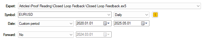
Figure 3: The test dates we used in the opening discussion of feedback controllers

Below, we have attached a screenshot of the previous performance levels established by the feedback controller. In our opening discussion, we provided this screenshot for the reader to contrast with the performance levels we aim to achieve today.

In the introduction of the article, we already gave a comprehensive summary of the key differences between the performance levels achieved previously and the performance levels we are aiming for now. The screenshot is included so that the reader also has the freedom to make their own queries.

Figure 4: A detailed analysis of the performance levels our benchmark established during its 5 year backtest

The equity curve shown below demonstrated promising potential in our opening discussion. However, as the reader will see, one of the examples presented today accelerated growth at a considerably more profitable rate than what was achieved in the past.

Figure 5: The equity curve we produced with the initial version of the feedback controller was already acceptable for our requirements

Z-Score (Standard Statistical Transformation)

The z-score transformation is a standard statistical technique that is generally considered a good first step for any dataset. The objective of this transformation is to preserve the different scales and dimensions that each column may take, as well as the ratios between them. This ensures your model can make comparisons in growth that are both meaningful and coherent.

Without accounting for scale, the model might make disproportionate judgments about growth in each column and its effect on the target. The z-score transformation solves this by subtracting the mean (the average value of each column) and then dividing by the standard deviation. As a result, each column ends with an average value of zero and a standard deviation of one.

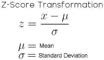
Figure 6: The mathematical formula for the statistical Z-score transformation we applied to our feedback controller input-data

   if(PositionsTotal() == 0)
     {
      //--- Find optimal solutions
      //--- Z-Score
       X = ((X - X.Mean())/X.Std());
      b_vector = y.MatMul(X.PInv());
      Print("Day Number: ",scenes+1);
      Print("Snapshot");
      Print(snapshots);
      Print("Input");
      Print(X);
      Print("Target");
      Print(y);
      Print("Coefficients");
      Print(b_vector);
      Print("Prediciton");
      prediction = b_vector.MatMul(snapshots.Col(scenes-1));
      Print("Expected Balance at next candle: ",prediction[4],". Expected Balance after 10 candles: ",prediction[8]);

As stated in the introduction of our article, the testing dates we use will remain the same across all tests. As shown in Figure 3 above, we will use the period starting from January 1, 2020, up until May 2025.

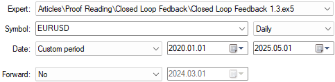
Figure 7: The backtest days we denoted above will be kept the same across all tests

As already mentioned, the Z-score transformation did not help improve our performance levels across the 5 year test. In fact, it negatively impacted our key performance metrics across the board.

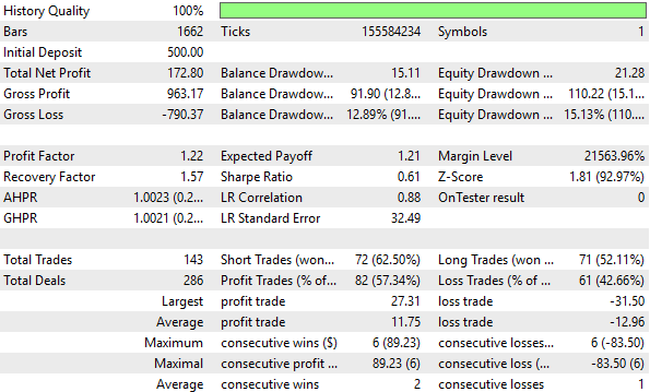
Figure 8: A detailed analysis of the performance metrics established by the z-score transformation shows no significant improvements

Our control setup from the previous discussion is more profitable than the equity curve demonstrated below by the transformation we have applied. Therefore we can conclude that this transformation destroyed the signal that was present in the raw data.

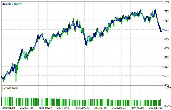
Figure 9: The equity curve produced by the z-score transformation failed to break higher than the equity curve we produced in the control setup

Unit Scaling (Standard Linear Algebra Transformation)

The idea of unit scaling is borrowed from the field of linear algebra. A bit of context is needed to fully understand this concept, since in our discussion we are not applying it in the standard way. Therefore, it is necessary to give a brief introduction for readers who may be encountering this idea for the first time.

Whenever we have a list of numbers—think of a simple array in MQL5 with, say, 10 numbers—there are many ways to measure how “big” that array is. In linear algebra, this size is referred to as the norm of an object. That object could be a vector or a matrix, but in this simple example we will consider only an array of numbers. From here on, I may use the words "array" and "vector" interchangeably, since they both refer to the same idea.

There are many ways to define how big an array is:

• We could measure it by how many elements it currently has.
• Additionally, we could measure it by how many elements it can hold at maximum capacity.
• To fully drive the point home, we could also consider measuring it by summing all the values of its current elements. 

The reader is intended to grasp that there are infinitely many ways we can measure "how big" an object is. The most appropriate measure, has a lot to do with the particular problem you are solving. But the most commonly used approach is to compute the sum of the elements the array has. However, if some values are positive and some are negative, simply adding them carelessly may cancel values out and return zero.

To avoid this, we can apply transformations before summing. For example, we might take the absolute value of each number, or square them before adding. These different approaches form a family of norms known as the Lp-norms.

One important norm to know from this family is the L1 norm, which is simply the sum of the absolute values of all elements in the array. Mathematically, this is shown in Figure 10 below.

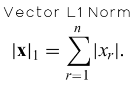
Figure 10: Defining the L1-Norm of a vector as the absolute sum of all its elements. 

After computing the L1 norm, we can then divide every value in the array by this norm. Doing so is called unit scaling in linear algebra, and it returns a normalized vector whose new norm equals 1. Meaning that if you take the norm of the vector again, the result will be exactly one.

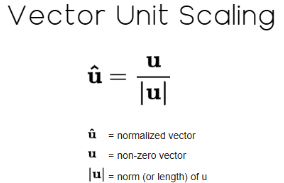
Figure 11: Unit scaling a vector is a standard transformation in linear algebra.

This is straightforward when dealing with vectors. However, our case is slightly different because we are working with a matrix, not just a vector. Recall from the beginning of our discussion that our data matrix, X, has 12 features. In this case, we must use the L1 norm of a matrix, which is not the same as the L1 norm of a vector, though the two are related.

According to the current MQL5 documentation, at the time of writing, the matrix L1 norm is defined as "MATRIX_NORM_P1 is the maximum vector p1-norm among horizontal matrix vectors."

While this definition is precise, it may not feel very intuitive at first, especially for readers considering all this for the first time. Therefore, I can paraphrase the documentation for the reader into more practical instructions that begin by first computing the L1 norm for each row of the matrix. Afterward, identify the row with the largest L1 norm. Then, that largest value becomes the L1 norm of the matrix. This is the idea defined by the MQL5 documentation, and it is defined mathematically by the notation illustrated in Figure 12 below:

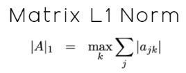
Figure 12: The L1 norm of a matrix is not the same as the L1 norm of a vector, though the 2 are related

Once the L1 norm has been computed, we finally divide every column in the dataset by this value, thereby applying a variation of unit scaling to the data.

   if(PositionsTotal() == 0)
     {
      //--- Find optimal solutions
      //--- We Must Take The Additional Steps Needed To Standardize & Scale Our Inputs
       X = X/X.Norm(MATRIX_NORM_P1);
      b_vector = y.MatMul(X.PInv());
      Print("Day Number: ",scenes+1);
      Print("Snapshot");
      Print(snapshots);
      Print("Input");
      Print(X);
      Print("Target");
      Print(y);
      Print("Coefficients");
      Print(b_vector);
      Print("Prediciton");
      prediction = b_vector.MatMul(snapshots.Col(scenes-1));
      Print("Expected Balance at next candle: ",prediction[4],". Expected Balance after 10 candles: ",prediction[8]);

As we stated before, we will keep all our backtest days the same across all tests to ensure fair comparisons.

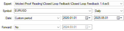
Figure 13: The backtest days we used for our tests have remained fixed across all examples

As the reader already knows, the unit scaling variation materially improved our performance levels over the benchmark, taking them to new heights we had not achieved before. This transformation clearly uncovered more signal within the data, helping our model detect more meaningful patterns. Not every transformation will work this way, but when one does, it produces measurable improvement—and measurable improvement is the only improvement that truly matters.

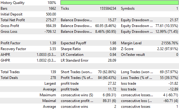
Figure 14: A detailed analysis of the performance levels attained by our improved feedback controller

When we examine the equity curve produced, we see that our profitability now reaches highs of 800, levels we could not achieve in our previous setup. Additionally, as mentioned in the introduction, the time it took for our account to grow from 500 to 700 has been reduced by almost a third—a remarkable increase in growth speed.

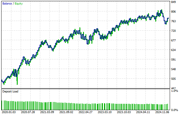
Figure 15: The new equity curve we have produced rises even faster than the old feedback controller we started with

Hybrid Approach (Unit Scaling & Z-score)

At this point in the article, as we stated in the introduction, there are no formalized rules for transformations. In this field, brute force testing is reasonably defensible because there is very little else we can do besides trying ideas and observing their performance. With that intuition in mind, we attempted to combine two transformations, hoping to achieve an even more powerful outcome.

  if(PositionsTotal() == 0)
     {
      //--- Find optimal solutions
      //--- We Must Take The Additional Steps Needed To Standardize & Scale Our Inputs
       X = X/X.Norm(MATRIX_NORM_P1);
       X = ((X-X.Mean())/X.Std());
      b_vector = y.MatMul(X.PInv());
      Print("Day Number: ",scenes+1);
      Print("Snapshot");
      Print(snapshots);
      Print("Input");
      Print(X);
      Print("Target");
      Print(y);
      Print("Coefficients");
      Print(b_vector);
      Print("Prediciton");
      prediction = b_vector.MatMul(snapshots.Col(scenes-1));
      Print("Expected Balance at next candle: ",prediction[4],". Expected Balance after 10 candles: ",prediction[8]);

Unfortunately, this hybrid approach proved largely unprofitable. Although it initially seemed promising, the combined transformations negatively affected all our key performance metrics.

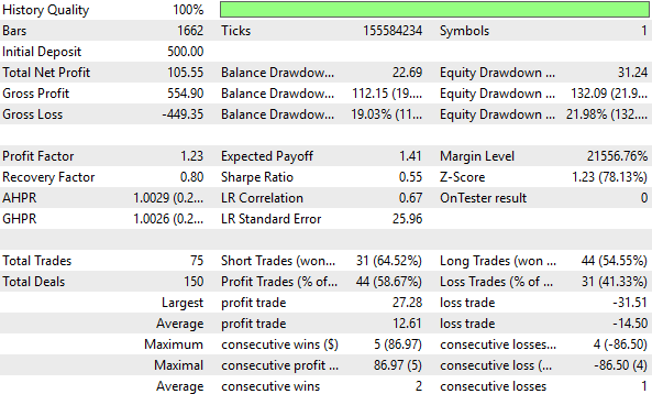
Figure 16: Our hybrid approach produced the worst performance levels we observed throughout this test

While the total proportion of profitable trades rose slightly—from 57.24% to 58.67% in the hybrid setup—this is not a meaningful improvement. Moreover, the equity curve produced by the hybrid strategy remains stuck between 500 and 600, failing to grow the account over time. Therefore, we can conclude that this transformation destroyed the signal in our input data and no longer exposes valuable relationships to our model.

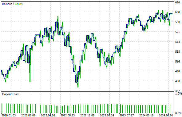
Figure 17: The equity curve we obtained no longer grows, and instead it appears to remain stuck in an unprofitable mode

Conclusion

From this discussion, the reader should walk away empowered with a new understanding of the pre-processing we apply to the data we feed our machine learning models. I hope the reader now views this step of the machine learning pipeline as a high-leverage tuning parameter—one that should be employed with diligence and persistence to truly yield benefits.

There are many transformations we can apply to a given dataset, and unfortunately, we often do not know which transformation is best, nor can we always tell if a particular transformation is helping. However, by employing a controlled framework—as demonstrated in this article—starting with a benchmark performance level and consistently testing ideas against it, we can uncover structure and patterns that may have been hidden in the original data.

It is therefore also important for the reader to continually expose themselves to as many transformations as possible, to test various approaches and discover what truly improves performance.