
Neural Networks in Trading: Reducing Memory Consumption with Adam-mini Optimization

Introduction
When we first started learning about neural networks, we discussed various approaches to optimizing model parameters. We use different approaches in our work. Most often I use the Adam method, which allows adaptively adjusting the optimal learning rate of each model parameter. However, this adaptability comes at a price. The Adam algorithm uses first and second-moment estimates for each model parameter, requiring the memory of the model itself. This memory consumption poses a significant issue when training large-scale models. In practice, maintaining an algorithm with such high memory demands often necessitates offloading computations to the CPU, increasing latency and slowing down the training process. Given these challenges, the search for new optimization methods or improvements to existing techniques has become increasingly relevant.
A promising solution was proposed in the paper "Adam-mini: Use Fewer Learning Rates To Gain More", published in July 2024. The authors introduced a modification of the Adam optimizer that maintains its performance while reducing memory consumption. The new optimizer, called Adam-mini, segments model parameters into blocks, assigns a single learning rate per block, and offers the following advantages:
- Lightweight: Adam-mini significantly reduces the number of learning rates used in Adam, which allows to reduce memory consumption by 45-50%.
- Efficiency: Despite lower resource usage, Adam-mini achieves performance comparable to or even better than standard Adam.
1. The Adam-mini Algorithm
The authors of Adam-mini analyze the role of v (the second-moment estimate) in Adam and explore ways to optimize it. In Adam, v provides an individual learning rate for each parameter. It has been observed that the Hessian matrix in Transformer architectures and other neural networks tends to exhibit a nearly block-diagonal structure. Moreover, each Transformer block demonstrates distinct eigenvalue distributions. As a result, Transformers require varying learning rates across different blocks to handle eigenvalue heterogeneity. This feature can be provided by v in Adam.
However, Adam does more than just assign learning rates to each block: it assigns them to every individual parameter. Note that the number of parameters far exceeds the number of blocks. This raises the question: Is it necessary to assign a unique learning rate to every parameter? If not, how much can we optimize?
The authors investigate this question across general optimization tasks and reach the following conclusions:
- Adam outperforms a single optimal learning rate method. This is expected since Adam applies different learning rates to different parameters.
- However, within a dense Hessian subblock, a single optimal learning rate can surpass Adam's performance.
- Therefore, applying optimal learning rates to a "block-wise" gradient descent approach enhances training efficiency.
For general optimization problems with a block-diagonal Hessian, increasing the number of learning rates does not necessarily bring additional benefits. Specifically, for each dense subblock, a single well-chosen learning rate is enough to achieve optimal performance.
Similar behavior is observed in Transformer-based architectures. The Adam-mini authors conduct experiments with a 4-layer Transformer and find that such models can achieve comparable or superior performance using significantly fewer learning rates than Adam.
This leaves an open question about how to efficiently determine optimal learning rates.
The goal of Adam-mini is to reduce memory usage for learning rates in Adam without requiring an exhaustive grid search.
Adam-mini consists of two steps. Step 1 is only required for initialization.
First, we divide the model parameters into blocks. In the case of Transformer, the authors of the method propose to group all Query and Keys entities based on attention heads. In all other cases, one second-moment estimate is used for each layer.
Embedding layers are treated separately. For embeddings, classic Adam remains preferable, since embeddings contain many zero values, their mean distribution differs significantly from the original variable's distribution.
In the second step of the algorithm, one learning rate is used for each block of parameters (outside the Embedding blocks). To effectively select the appropriate learning rate in each block, Adam-mini simply replaces the squared gradient in Adam with its mean value. The authors of the method apply a moving average to these mean values, as in the classical Adam.
By design, Adam-mini reduces the number of learning rates in Transformers from one per parameter to the sum of the embedding layer size, output layer size, and the number of non-embedding blocks. The extent of memory savings depends on the proportion of non-embedding parameters in the model.
Adam-mini can achieve higher throughput compared to Adam, especially with limited hardware resources. There are two reasons for this. First, Adam-mini does not add any additional computational load in its update rules. Besides, Adam-mini significantly reduces the number of square root and tensor division operations which are used in Adam.
Second, due to the lower memory usage, Adam-mini can support larger batch sizes on GPU, while simultaneously reducing GPU-to-CPU communication, another major training bottleneck.
These improvements enable Adam-mini to accelerate pretraining of large models by reducing both memory consumption and computational costs.
Adam-mini projects a learning rate for each dense Hessian subblock using the v Adam mean within each block. This approach can be computationally efficient but may not be fully optimal. However, the current design is sufficient to achieve performance comparable to or even slightly better than Adam, while significantly lowering memory requirements.
2. Implementing in MQL5
After considering the theoretical aspects of the Adam-mini method, let us move on to the practical part of our article. In this part, we implement our own vision of the described approaches using MQL5.
Please note that this work differs significantly from what we did in previous articles. Usually, we implement new approaches within the framework of a single layer class in our model. However, in this case, we need to introduce modifications across previously developed classes. This is because each of these classes contains an overridden or inherited updateInputWeights method, which defines the algorithm for updating model parameters at the layer level.
Of course, some updateInputWeights methods belong to complex architectural components where we simply call the corresponding methods of nested objects. A good example is the Decoder, discussed in our previous article. In such cases, the algorithm remains independent of the chosen optimization method.
bool CNeuronSTNNDecoder::updateInputWeights(CNeuronBaseOCL *NeuronOCL, CBufferFloat *Context)
  {
   if(!cEncoder.UpdateInputWeights(NeuronOCL, Context))
      return false;
   if(!CNeuronMLCrossAttentionMLKV::updateInputWeights(cEncoder.AsObject(), Context))
      return false;
//---
   return true;
  }
Continuing down the hierarchy of function calls, we always reach the fundamental "workhorses" where the main parameter update algorithm is implemented.
2.1 Implementing Adam-mini in the Basic Fully Connected Layer
One such class is our basic fully connected layer, CNeuronBaseOCL. Therefore, our work will begin here.
It's important to remember that most of the computational tasks are implemented on the GPU side for parallel processing. This process is no exception. Consequently, we will interact with an OpenCL program, where we will create a new kernel called UpdateWeightsAdamMini.
Before diving into the actual code, let's briefly discuss our architectural solution.
Firstly, the main difference between the Adam-mini optimization method and classic Adam lies primarily in the calculation of the second-order moment v. Instead of using the gradient of each individual parameter, the authors of Adam-mini suggest using the average value of a group. The algorithm for computing this simple average is straightforward. By doing so, we free up a significant amount of memory, as only a single value for the second-order moment is stored for each group.
On the other hand, we don't want to repeat the calculation of the mean for the entire block in every individual thread. Recall that, for the fully connected layer, the Adam-mini method suggests using just one learning rate. Thus, recalculating the mean of the gradient for every parameter of the layer in each thread does not seem efficient, to say the least. Moreover, considering the high cost of accessing global memory, the best solution is to parallelize this process across multiple threads while minimizing global memory access. However, this immediately raises the issue of how to organize data exchange between threads.
In previous articles, we have already learned how to exchange data within a local group with thread synchronization. However, organizing the entire parameter update process of a layer within a single local group doesn't seem particularly attractive. Therefore, in this implementation, I decided to increase the number of second-order moments calculated to match the size of the result tensor.
As we know, the number of parameters in a fully connected layer is the product of the size of the input tensor and the size of the result tensor. Additionally, the use of a bias parameter for each neuron adds the number of parameters equal to the size of the result tensor. Classic Adam stores an equal number of values for both the first and second moments. In the Adam-mini implementation, we significantly reduce the number of second-order moment values stored.
![]()
Now let's discuss a little bit the process of calculating the average value of the second order moment. The error gradient of 1 parameter is equal to the product of the error gradient at the layer output (corrected by the derivative of the activation function) and the corresponding input value.
![]()
Thus, the average of the squared gradients can be computed as follows:
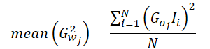
Since our implementation calculates the average gradient for a single neuron in the result layer, we can factor out the gradient of that neuron from the equation.
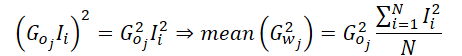
This means that, in our implementation of the average second-order moment, we only need to compute the average squared values of the input data. By doing so, we eliminate the need for frequent access to the global memory buffer that stores the output gradient. After obtaining this mean value, we then take the output gradient only once, square it, and multiply it by the computed average. Finally, we simply distribute the resulting value across the local group for further calculations.
Now that we have a clear understanding of the computational process, we can proceed with implementing it in the UpdateWeightsAdamMini kernel. The parameters of this kernel are nearly identical to those of the classic Adam kernel. These include 5 data buffers and 3 constants:
- matrix_w — matrix of layer parameters;
- matrix_g — the error gradient tensor at the layer output;
- matrix_i — input data buffer;
- matrix_m — the first-order moment tensor;
- matrix_v — the second-order moment tensor;
- l — learning rate;
- b1 — first-order moment smoothing coefficient (ß1);
- b2 — second-order moment smoothing coefficient (ß2);
__kernel void UpdateWeightsAdamMini(__global float *matrix_w,
                                    __global const float *matrix_g,
                                    __global const float *matrix_i,
                                    __global float *matrix_m,
                                    __global float *matrix_v,
                                    const float l,
                                    const float b1,
                                    const float b2
                                   )
  {
//--- inputs
   const size_t i = get_local_id(0);
   const size_t inputs = get_local_size(0) - 1;
//--- outputs
   const size_t o = get_global_id(1);
   const size_t outputs = get_global_size(1);
The kernel execution is planned in a 2-dimensional task space. The first dimension corresponds to the number of input values plus the offset element. The second is the size of the result tensor. In the kernel body we first identify the thread in both dimensions.
Note that we combine threads into workgroups along 1 dimension of the task space.
Next, we organize an array in the local context memory for exchanging data between the threads of the workgroup.
   __local float temp[LOCAL_ARRAY_SIZE];
   const int ls = min((uint)LOCAL_ARRAY_SIZE, (uint)inputs);
The next step is to compute the average squared value of the input data. Since the input data buffer will also be needed for the calculation of the first-order moment, each thread will first retrieve the corresponding value from the global input data buffer.
const float inp = (i < inputs ? matrix_i[i] : 1.0f);
Then, we will implement a loop with thread synchronization, where each thread will add the squared value of its input data element to a local array.
   int count = 0;
   do
     {
      if(count == (i / ls))
        {
         int shift = i % ls;
         temp[shift] = (count == 0 ? 0 : temp[shift]) + ((isnan(inp) || isinf(inp)) ? 0 : inp*inp);
        }
      count++;
      barrier(CLK_LOCAL_MEM_FENCE);
     }
   while(count * ls < inputs);
After that we sum the values of the elements of the local array.
//--- sum
   count = (ls + 1) / 2;
   do
     {
      if(i < count && (i + count) < ls)
        {
         temp[i] += temp[i + count];
         temp[i + count] = 0;
        }
      count = (count + 1) / 2;
      barrier(CLK_LOCAL_MEM_FENCE);
     }
   while(count > 1);
Within one thread, we implement the calculation of the second-order moment and save it in the local array element with index 0.
Also, we remember that accessing a local memory array is much faster than accessing a global memory buffer. Therefore, to reduce the number of global memory access operations, we take the error gradient at the level of the current layer results and save it in the local array element with index 1. Thus, the remaining elements of the workgroup, when performing subsequent operations, will take the value from the local memory instead of accessing global memory.
Make sure to synchronize the work of the workgroup threads.
//--- calc v
   if(i == 0)
     {
      temp[1] = matrix_g[o];
      if(isnan(temp[1]) || isinf(temp[1]))
         temp[1] = 0;
      temp[0] /= inputs;
      if(isnan(temp[0]) || isinf(temp[0]))
         temp[0] = 1;
      float v = matrix_v[o];
      if(isnan(v) || isinf(v))
         v = 1;
      temp[0] = b2 * v + (1 - b2) * pow(temp[1], 2) * temp[0];
      matrix_v[o] = temp[0];
     }
   barrier(CLK_LOCAL_MEM_FENCE);
Note that we immediately save the second-order moment value in the global data buffer. This simple step helps eliminate unnecessary global memory accesses from other threads within the workgroup, reducing delays caused by simultaneous access to the same global buffer element from multiple threads.
Next, our algorithm follows the operations of the classic Adam method. At this stage, we determine the offset in the tensor of trainable parameters and load the current value of the analyzed parameter from the global memory buffer.
   const int wi = o * (inputs + 1) + i;
   float weight = matrix_w[wi];
   if(isnan(weight) || isinf(weight))
      weight = 0;
We calculate the value of the first order moment.
   float m = matrix_m[wi];
   if(isnan(m) || isinf(m))
      m = 0;
//--- calc m
   m = b1 * m + (1 - b1) * temp[1] * inp;
   if(isnan(m) || isinf(m))
      m = 0;
Determine the size of the parameter adjustment.
   float delta = l * (m / (sqrt(temp[0]) + 1.0e-37f) - (l1 * sign(weight) + l2 * weight));
   if(isnan(delta) || isinf(delta))
      delta = 0;
After that, we correct the parameter value and save its new value in the global data buffer.
   if(delta > 0)
      matrix_w[wi] = clamp(weight + delta, -MAX_WEIGHT, MAX_WEIGHT);
   matrix_m[wi] = m;
  }
Here we save the value of the first order moment and complete the kernel operation.
After making changes on the OpenCL side, we need to make a number of edits to the main program. First of all, we will add a new optimization method to our enumeration.
//+------------------------------------------------------------------+
/// Enum of optimization method used                                 |
//+------------------------------------------------------------------+
enum ENUM_OPTIMIZATION
  {
   SGD,        ///< Stochastic gradient descent
   ADAM,       ///< Adam
   ADAM_MINI   ///< Adam-mini
  };
After that we will make changes to the CNeuronBaseOCL::updateInputWeights method. Here in the variable declaration block we will add an array describing the sizes of the workgroup, local_work_size (underlined in the code below). At this stage we do not assign values to it, since they will only be needed when using the corresponding optimization method.
bool CNeuronBaseOCL::updateInputWeights(CNeuronBaseOCL *NeuronOCL)
  {
   if(CheckPointer(OpenCL) == POINTER_INVALID || CheckPointer(NeuronOCL) == POINTER_INVALID)
      return false;
   uint global_work_offset[2] = {0, 0};
   uint global_work_size[2], local_work_size[2];
   global_work_size[0] = Neurons();
   global_work_size[1] = NeuronOCL.Neurons() + 1;
   uint rest = 0;
   float lt = lr;
Next comes the branching of the algorithm depending on the chosen method for optimizing the model parameters. We will use the same algorithms for queuing kernels for execution as we used in the previously considered optimization methods, so we will not dwell on them.
   switch(NeuronOCL.Optimization())
     {
      case SGD:
.........
.........
.........
         break;
      case ADAM:
........
........
........
         break;
Let's just look at the added code. First we pass the parameters necessary for the kernel to work correctly.
      case ADAM_MINI:
         if(!OpenCL.SetArgumentBuffer(def_k_UpdateWeightsAdamMini, def_k_wuam_matrix_w,
                                                           NeuronOCL.getWeightsIndex()))
            return false;
         if(!OpenCL.SetArgumentBuffer(def_k_UpdateWeightsAdamMini, def_k_wuam_matrix_g,
                                                                    getGradientIndex()))
            return false;
         if(!OpenCL.SetArgumentBuffer(def_k_UpdateWeightsAdamMini, def_k_wuam_matrix_i,
                                                            NeuronOCL.getOutputIndex()))
            return false;
         if(!OpenCL.SetArgumentBuffer(def_k_UpdateWeightsAdamMini, def_k_wuam_matrix_m,
                                                     NeuronOCL.getFirstMomentumIndex()))
            return false;
         if(!OpenCL.SetArgumentBuffer(def_k_UpdateWeightsAdamMini, def_k_wuam_matrix_v,
                                                    NeuronOCL.getSecondMomentumIndex()))
            return false;
         lt = (float)(lr * sqrt(1 - pow(b2, (float)t)) / (1 - pow(b1, (float)t)));
         if(!OpenCL.SetArgument(def_k_UpdateWeightsAdamMini, def_k_wuam_l, lt))
            return false;
         if(!OpenCL.SetArgument(def_k_UpdateWeightsAdamMini, def_k_wuam_b1, b1))
            return false;
         if(!OpenCL.SetArgument(def_k_UpdateWeightsAdamMini, def_k_wuam_b2, b2))
            return false;
After that, we will define the task spaces of the global work of the kernel and a separate work group.
         global_work_size[0] = NeuronOCL.Neurons() + 1;
         global_work_size[1] = Neurons();
         local_work_size[0] = global_work_size[0];
         local_work_size[1] = 1;
Note that in the first dimension, both globally and for the workgroup, we specify a value that is 1 element larger than the size of the input data layer. This is our offset parameter. But in the second dimension we globally indicate the number of elements in the current neural layer. For the workgroup, we indicate 1 element in this dimension. This corresponds to the operations of the workgroup within 1 neuron of the current layer.
After the preparatory work has been completed, the kernel is placed in the execution queue.
         ResetLastError();
         if(!OpenCL.Execute(def_k_UpdateWeightsAdamMini, 2, global_work_offset, global_work_size,
                                                                                local_work_size))
           {
            printf("Error of execution kernel UpdateWeightsAdamMini: %d", GetLastError());
            return false;
           }
         t++;
         break;
      default:
         return false;
         break;
     }
//---
   return true;
  }
And we add an exit with a negative result in case an incorrect optimization method is specified.
With this, we complete the implementation of the parameter update method for the basic fully connected layer CNeuronBaseOCL::updateInputWeights. However, let's recall the primary goal of these modifications: reducing memory consumption when using the Adam optimization method. Therefore, we must also adjust the CNeuronBaseOCL::Init initialization method, to reduce the size of the second-order moment buffer when the Adam-mini optimization method is selected. Since these changes are minimal and targeted, I will not provide a full description of the method algorithm in this article. Instead, I will present only the initialization block for the corresponding buffer.
         if(CheckPointer(SecondMomentum) == POINTER_INVALID)
           {
            SecondMomentum = new CBufferFloat();
            if(CheckPointer(SecondMomentum) == POINTER_INVALID)
               return false;
           }
         if(!SecondMomentum.BufferInit((optimization == ADAM_MINI ? numOutputs : count), 0))
            return false;
         if(!SecondMomentum.BufferCreate(OpenCL))
            return false;
You can find the full implementation of this method in the attached files, along with the complete code for all the programs used in preparing this article.
2.2 Adam-mini in the Convolutional Layer
Another fundamental building block widely used in various architectures, including Transformer, is the convolutional layer.
Integrating the Adam-mini optimization method into its functionality has some unique aspects, primarily due to the specific nature of convolutional layers. Unlike fully connected layers, where each trainable parameter is responsible for transmitting the value of only one input neuron to only one neuron in the current layer, convolutional layers typically have fewer parameters, but each parameter is used more extensively.
Additionally, it's important to note that we use convolutional layers to generate Query, Key, and Value entities in Transformer algorithms. These entities require a specialized implementation of the Adam-mini method.
All these factors must be considered when implementing the Adam-mini method within a convolutional layer.
As with the fully connected layer, we start by implementing the method on the OpenCL side. Here, we create the UpdateWeightsConvAdamMini kernel. In addition to the familiar variables, this kernel introduces two new constants: the sequence length of the input data and the stride of the convolution window.
__kernel void UpdateWeightsConvAdamMini(__global float *matrix_w,
                                        __global const float *matrix_i,
                                        __global float *matrix_m,
                                        __global float *matrix_v,
                                        const int inputs,
                                        const float l,
                                        const float b1,
                                        const float b2,
                                        int step
                                       )
  {
//--- window in
   const size_t i = get_global_id(0);
   const size_t window_in = get_global_size(0) - 1;
//--- window out
   const size_t f = get_global_id(1);
   const size_t window_out = get_global_size(1);
//--- head window out
   const size_t f_h = get_local_id(1);
   const size_t window_out_h = get_local_size(1);
//--- variable
   const size_t v = get_global_id(2);
   const size_t variables = get_global_size(2);
Please note that in the kernel parameters, we do not specify the size of the input data window and the number of filters used. These parameters, along with two others, are moved to the task space, which is an important aspect to consider.
This kernel is designed to be executed in a three-dimensional task space: The first dimension corresponds to the input window size plus one additional element for bias. Here, we can observe a certain similarity with the task space of the fully connected layer.
The second dimension represents the number of filters used, which logically corresponds to the output dimensionality of the fully connected layer.
As for the workgroups, we will not create them for each individual convolution filter, but we will group them by the attention heads of the Transformer architecture.
Please note that the user can only specify one convolution filter for each head. In this case, each convolution filter will receive an individual learning rate similar to our implementation of a fully connected layer.
The third dimension is introduced to handle multimodal time series, where individual unitary sequences have their own convolutional filters. Separate second-order moments are also created for them to enable adaptive learning rates.
A distinction must be made between "attention heads" and "unitary time series", as they should not be confused. While they may appear similar, they serve different roles. Unitary time series divide the input tensor. Attention heads divide the output tensor.
Inside the kernel, after identifying the thread in all dimensions of the task space, we define the main offset constants in the global data buffers.
//--- constants
   const int total = (inputs - window_in + step - 1) / step;
   const int shift_var_in = v * inputs;
   const int shift_var_out = v * total * window_out;
   const int shift_w = (f + v * window_out) * (window_in + 1) + i;
We create a local array for the workgroup data exchange.
   __local float temp[LOCAL_ARRAY_SIZE];
   const int ls = min((uint)window_in, (uint)LOCAL_ARRAY_SIZE);
After the preparatory work, we will collect error gradients for each parameter.
//--- calc gradient
   float grad = 0;
   for(int t = 0; t < total; t++)
     {
      if(i != window_in && (i + t * window_in) >= inputs)
         break;
      float gt = matrix_g[t * window_out + f + shift_var_out] *
                 (i == window_in ? 1 : matrix_i[i + t * step + shift_var_in]);
      if(!(isnan(gt) || isinf(gt)))
         grad += gt;
     }
Note that in this case, each global thread completely collects error gradients from all elements it influences. Unlike the fully connected layer, here we immediately multiply the value of the input data element by the corresponding error gradient of the results.
Next, we accumulate the computed error gradients to sum their squared values within a local array, but now at the workgroup level. To achieve this, we implement a nested loop structure with mandatory thread synchronization. The outer loop corresponds to the number of filters within the workgroup. The inner loop gathers the error gradients from all parameters of a single filter.
//--- calc sum grad
   int count;
   for(int h = 0; h < window_out_h; h++)
     {
      count = 0;
      do
        {
         if(h == f_h)
           {
            if(count == (i / ls))
              {
               int shift = i % ls;
               temp[shift] = ((count == 0 && h == 0) ? 0 : temp[shift]) +
                             ((isnan(grad) || isinf(grad)) ? 0 : grad * grad);
              }
           }
         count++;
         barrier(CLK_LOCAL_MEM_FENCE);
        }
      while((count * ls) < window_in);
     }
Then we sum the values of the local array.
   count = (ls + 1) / 2;
   do
     {
      if(i < count && (i + count) < ls && f_h == 0)
        {
         temp[i] += temp[i + count];
         temp[i + count] = 0;
        }
      count = (count + 1) / 2;
      barrier(CLK_LOCAL_MEM_FENCE);
     }
   while(count > 1);
We also will determine the value of the second-order moment of the current group.
//--- calc v
   if(i == 0 && f_h == 0)
     {
      temp[0] /= (window_in * window_out_h);
      if(isnan(temp[0]) || isinf(temp[0]))
         temp[0] = 1;
      int head = f / window_out_h;
      float v = matrix_v[head];
      if(isnan(v) || isinf(v))
         v = 1;
      temp[0] = clamp(b2 * v + (1 - b2) * temp[0], 1.0e-6f, 1.0e6f);
      matrix_v[head] = temp[0];
     }
   barrier(CLK_LOCAL_MEM_FENCE);
Next, we repeat the algorithm of the classical Adam method. Here we define the first-order moment.
//--- calc m
   float mt = clamp(b1 * matrix_m[shift_w] + (1 - b1) * grad, -1.0e5f, 1.0e5f);
   if(isnan(mt) || isinf(mt))
      mt = 0;
We adjust the value of the analyzed parameter.
float weight = clamp(matrix_w[shift_w] + l * mt / sqrt(temp[0]), -MAX_WEIGHT, MAX_WEIGHT);
And we save the obtained values.
   if(!(isnan(weight) || isinf(weight)))
      matrix_w[shift_w] = weight;
   matrix_m[shift_w] = mt;
  }
After creating the kernel on the OpenCL side, we are moving on to work on the main program. As in the case of a fully connected layer, we implement the call of the above created kernel in the CNeuronConvOCL::updateInputWeights method. The algorithm for calling it is similar to the one presented above for a fully connected layer. For a normal convolutional layer, we use one filter for each attention head and use one unitary sequence. Thus, the dimension of the task space will take the following form.
   uint global_work_offset_am[3] = { 0, 0, 0 };
   uint global_work_size_am[3] = { iWindow + 1, iWindowOut, iVariables };
   uint local_work_size_am[3] = { global_work_size_am[0], 1, 1 };
You can find the full implementation of this method in the attached files,
However, I would like to add a few words about using the created kernel within the implementation of classes that utilize the Transformer architecture. As an example, let's consider the CNeuronMLMHAttentionOCL class. This class serves as the parent class for building a variety of other algorithms.
It is important to note that the CNeuronMLMHAttentionOCL class does not contain convolutional layers in the traditional sense. Instead, it organizes buffer arrays and overrides all relevant methods. The parameter updates for the convolutional layers are handled in the ConvolutionUpdateWeights method. Since this method is used for managing various convolutional layers, we will add two additional parameters: the number of attention heads (heads) and the number of unitary sequences (variables). To avoid potential issues with accessing this method from other classes, these new parameters will be given default values.
bool CNeuronMLMHAttentionOCL::ConvolutuionUpdateWeights(CBufferFloat *weights,
                                                        CBufferFloat *gradient,
                                                        CBufferFloat *inputs,
                                                        CBufferFloat *momentum1,
                                                        CBufferFloat *momentum2,
                                                        uint window, uint window_out,
                                                        uint step = 0, uint heads = 0,
                                                        uint variables = 1)
  {
   if(CheckPointer(OpenCL) == POINTER_INVALID || CheckPointer(weights) == POINTER_INVALID ||
      CheckPointer(gradient) == POINTER_INVALID || CheckPointer(inputs) == POINTER_INVALID  ||
      CheckPointer(momentum1) == POINTER_INVALID)
      return false;
In the method body, we first check the pointers to the data buffers that the method receives as parameters from the caller.
Next we check the value of the convolution window stride (step) parameter. If it is equal to "0", then we take the step equal to the convolution window.
   if(step == 0)
      step = window;
Note that in this case we are using unsigned data type for the parameters. Therefore, they cannot contain negative values. We leave control over inflated parameter values to the user.
We then define task spaces. In this case, the kernel of the Adam-mini optimization method uses a 3-dimensional task space, which differs from the one-dimensional one used by other optimization methods. Therefore, we allocate separate arrays to indicate it.
   uint global_work_offset[1] = {0};
   uint global_work_size[1];
   global_work_size[0] = weights.Total();
   uint global_work_offset_am[3] = {0, 0, 0};
   uint global_work_size_am[3] = {window, window_out, 1};
   uint local_work_size_am[3] = {window, (heads > 0 ? window_out / heads : 1), variables};
Let's take a look at the second dimension of the workgroup task space. If the number of attention heads is not specified in the method parameters, then each filter will have a separate learning rate. If the number of attention heads is provided, we compute the number of filters per attention head by dividing the total number of filters by the number of attention heads.
This approach was chosen to accommodate various usage scenarios of this method. Within the CNeuronMLMHAttentionOCL class, convolutional layers are used both to form the Query, Key, and Value entities, as well as for data projection (within the multi-head attention downsampling layer and the FeedForward block).
The next step is to separate the algorithm depending on the optimization method used for the model parameters. Just like in the fully connected layer algorithm discussion, we won’t dive into the details of how previously implemented optimization methods work. We'll consider only the Adam-mini method block.
   if(weights.GetIndex() < 0)
      return false;
   float lt = 0;
   switch(optimization)
     {
      case SGD:
........
........
........
         break;
      case ADAM:
........
........
........
         break;
      case ADAM_MINI:
         if(CheckPointer(momentum2) == POINTER_INVALID)
            return false;
         if(gradient.GetIndex() < 0)
            return false;
         if(inputs.GetIndex() < 0)
            return false;
         if(momentum1.GetIndex() < 0)
            return false;
         if(momentum2.GetIndex() < 0)
            return false;
Here we check the relevance of pointers to data buffers in the OpenCL context. After that we will pass all the necessary parameters to the kernel.
         if(!OpenCL.SetArgumentBuffer(def_k_UpdateWeightsConvAdamMini, def_k_wucam_matrix_w,
                                                                         weights.GetIndex()))
            return false;
         if(!OpenCL.SetArgumentBuffer(def_k_UpdateWeightsConvAdamMini, def_k_wucam_matrix_g,
                                                                        gradient.GetIndex()))
            return false;
         if(!OpenCL.SetArgumentBuffer(def_k_UpdateWeightsConvAdamMini, def_k_wucam_matrix_i,
                                                                          inputs.GetIndex()))
            return false;
         if(!OpenCL.SetArgumentBuffer(def_k_UpdateWeightsConvAdamMini, def_k_wucam_matrix_m,
                                                                       momentum1.GetIndex()))
            return false;
         if(!OpenCL.SetArgumentBuffer(def_k_UpdateWeightsConvAdamMini, def_k_wucam_matrix_v,
                                                                       momentum2.GetIndex()))
            return false;
         lt = (float)(lr * sqrt(1 - pow(b2, t)) / (1 - pow(b1, t)));
         if(!OpenCL.SetArgument(def_k_UpdateWeightsConvAdamMini, def_k_wucam_inputs,
                                                                            inputs.Total()))
            return false;
         if(!OpenCL.SetArgument(def_k_UpdateWeightsConvAdamMini, def_k_wucam_l, lt))
            return false;
         if(!OpenCL.SetArgument(def_k_UpdateWeightsConvAdamMini, def_k_wucam_b1, b1))
            return false;
         if(!OpenCL.SetArgument(def_k_UpdateWeightsConvAdamMini, def_k_wucam_b2, b2))
            return false;
         if(!OpenCL.SetArgument(def_k_UpdateWeightsConvAdamMini, def_k_wucam_step, (int)step))
            return false;
We have already shown the task space earlier. And now we just need to put the kernel into the execution queue.
         ResetLastError();
         if(!OpenCL.Execute(def_k_UpdateWeightsConvAdamMini, 3, global_work_offset_am,
                                              global_work_size_am, local_work_size_am))
           {
            string error;
            CLGetInfoString(OpenCL.GetContext(), CL_ERROR_DESCRIPTION, error);
            printf("Error of execution kernel %s Adam-Mini: %s", __FUNCSIG__, error);
            return false;
           }
         t++;
         break;
      //---
      default:
         printf("Error of optimization type %s: %s", __FUNCSIG__, EnumToString(optimization));
         return false;
     }
We will also add an error message when specifying an incorrect type of parameter optimization.
The further code of the method in terms of normalizing the model parameters remained unchanged.
   global_work_size[0] = window_out;
   OpenCL.SetArgumentBuffer(def_k_NormilizeWeights, def_k_norm_buffer, weights.GetIndex());
   OpenCL.SetArgument(def_k_NormilizeWeights, def_k_norm_dimension, (int)window + 1);
   if(!OpenCL.Execute(def_k_NormilizeWeights, 1, global_work_offset, global_work_size))
     {
      string error;
      CLGetInfoString(OpenCL.GetContext(), CL_ERROR_DESCRIPTION, error);
      printf("Error of execution kernel %s Normalize: %s", __FUNCSIG__, error);
      return false;
     }
//---
   return true;
  }
Additionally, in the initialization methods of the above-mentioned classes, we modify the size of the data buffers created to store second-order moments, similarly to the algorithm presented when describing the changes in the fully connected layer. However, I will not delve into this in the article. These are just minor edits that you can explore in the attachment.
3. Testing
The implementation of the Adam-mini method in two base classes of our models has been described above. Now it's time to evaluate the effectiveness of the proposed approach.
In this article, we introduced a new optimization method. To assess the effectiveness of this optimization method, it's logical to observe the training process of a model using different optimization techniques.
For this experiment, I took the models from the TPM algorithm article and modified the architecture of the models, changing only the method for optimizing parameters.
Needless to say, when using this approach, all training programs, datasets, and the training process remain unchanged.
To remind you, the models were trained on historical data for the entire year of 2023, using EURUSD with the H1 timeframe. The parameters of all indicators were set to default.
When testing the trained model, we achieved results similar to the model trained with the classic Adam method. The testing results on January 2024 data are presented below.

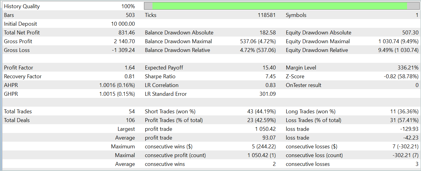
It's important to note that the main goal of the Adam-mini optimization method is to reduce memory consumption without compromising the quality of training. The proposed method successfully meets this goal.
Conclusion
In this article, we introduced a new optimization method Adam-mini, which was developed to reduce memory usage and increase throughput when training large language models. Adam-mini achieves this by reducing the number of required learning rates to the sum of the embedding layer size, the results layer size, and the number of blocks in other layers. Its simplicity, flexibility, and efficiency make it a promising tool for broad application in deep learning.
The practical part of the article demonstrated the integration of the proposed method into the basic types of neural layers. The results of the tests confirm the improvements stated by the authors of the method.
References
Programs used in the article
| # | Name | Type | Description |
|---|---|---|---|
| 1 | Research.mq5 | Expert Advisor | Example collection EA |
| 2 | ResearchRealORL.mq5 | Expert Advisor | EA for collecting examples using the Real-ORL method |
| 3 | Study.mq5 | Expert Advisor | Model training EA |
| 4 | StudyEncoder.mq5 | Expert Advisor | Encoder training EA |
| 5 | Test.mq5 | Expert Advisor | Model testing EA |
| 6 | Trajectory.mqh | Class library | System state description structure |
| 7 | NeuroNet.mqh | Class library | A library of classes for creating a neural network |
| 8 | NeuroNet.cl | Code Base | OpenCL program code library |
Translated from Russian by MetaQuotes Ltd.
Original article: https://www.mql5.com/ru/articles/15352
Warning: All rights to these materials are reserved by MetaQuotes Ltd. Copying or reprinting of these materials in whole or in part is prohibited.
This article was written by a user of the site and reflects their personal views. MetaQuotes Ltd is not responsible for the accuracy of the information presented, nor for any consequences resulting from the use of the solutions, strategies or recommendations described.

- Free trading apps
- Over 8,000 signals for copying
- Economic news for exploring financial markets
You agree to website policy and terms of use
Hello, I wanted to ask you, when I run Study, I get Error of execution kernel UpdateWeightsAdamMini: 5109, what is the reason and how to solve it, thank you very much in advance.
Good afternoon, can you post the execution log and architecture of the model you are using?
Hello, I am sending you the Studio Encode and Study recordings. As for the architecture, it is almost the same as you presented, except that the number of candles in the study is 12 and the data of these candles is 11. Also in the output layer I have only 4 parameters.
Buenas tardes, ¿puedes publicar el registro de ejecución y la arquitectura del modelo utilizado?