
Neural Networks in Trading: Contrastive Pattern Transformer

Introduction
When analyzing market situations using machine learning, we often focus on individual candlesticks and their attributes, overlooking candlestick patterns that frequently provide more meaningful information. Patterns represent stable candlestick structures that emerge under similar market conditions and can reveal critical behavioral trends.
Previously, we explored the Molformer framework, borrowed from the domain of molecular property prediction. The authors of Molformer combined atomic and motif representations into a single sequence, enabling the model to access structural information about the analyzed data. However, this approach introduced the complex challenge of separating dependencies between nodes of different types. Fortunately, alternative methods have been proposed that avoid this issue.
One such example is the Atom-Motif Contrastive Transformer (AMCT), introduced in the paper "Atom-Motif Contrastive Transformer for Molecular Property Prediction". To integrate the two levels of interactions and enhance the representational capacity of molecules, the authors of AMCT proposed to apply contrastive learning between atom and motif representations. Since atom and motif representations of a molecule are essentially two different views of the same entity, they naturally align during training. This alignment allows them to provide mutual self-supervised signals, thereby improving the robustness of the learned molecular representations.
It has been observed that identical motifs across different molecules tend to exhibit similar chemical properties. This suggests that identical motifs should have consistent representations across molecules. Consequently, using contrastive loss maximizes the alignment of identical motifs in different molecules, resulting in more distinguishable motif representations.
Furthermore, to effectively identify the motifs that are critical for determining each molecule's properties, the authors incorporated an attention mechanism that integrates property information through a cross-attention module. Specifically, the cross-attention module captures dependencies between molecular property embeddings and motif representations. As a result, key motifs can be identified based on cross-attention weights.
1. The AMCT Algorithm
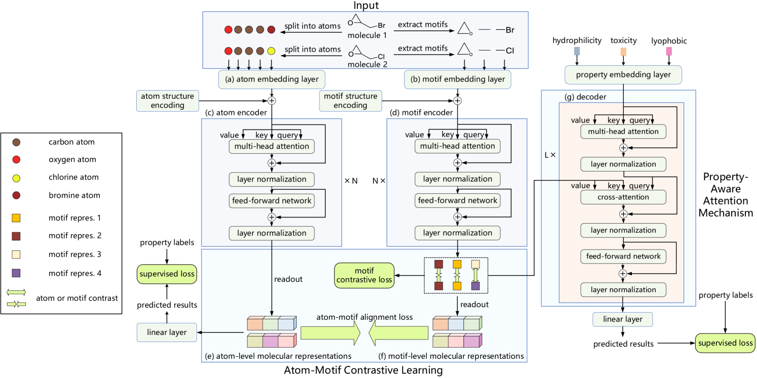
The molecular descriptions input into the model are initially decomposed into a set of atoms and segmented into a set of motifs. These resulting sequences are then fed into parallel atom and motif encoding layers, which generate the respective embeddings. Two independent Encoders are used to obtain molecular representations at the atom and motif levels. Also, a Decoder and a fully connected layer are used to produce the predicted outputs. During model training, the loss functions include atom-motif alignment loss, motif-level contrastive loss, and property prediction loss.
In the atom encoding process, we first obtain the atom embeddings. These embeddings are then processed by the atom encoder to extract dependencies between individual atoms within the molecule. The output is a molecular representation at the atom level.
The authors of AMCT use node centrality to encode structural information between atoms, specifically the bonding relationships of atoms within a molecule. Since centrality is applied to each atom, it is simply added to the atom embeddings.
While the atom-level dependencies effectively capture low-level details, they overlook high-level structural information among different atoms. Consequently, this approach may be insufficient for accurately predicting molecular properties. To address this problem, the AMCT framework introduces a parallel pathway for molecular representation at the motif level. In motif encoding, motifs are first extracted from the original dataset and then transformed into embeddings. These embeddings are processed by the motif encoder to capture dependencies between motifs.
The AMCT framework also uses centrality to encode structural information between motifs, which is added to their corresponding embeddings.
To explore the additional information provided by motifs, the framework considers the similarity relationships between molecular representations at the atom and motif levels. Since atom and motif representations of a single molecule are, in essence, two different views of the same entity, they naturally align to generate self-supervised signals during model training. The authors employ Kullback-Leibler divergence to align the two representations.
Because atom-motif alignment loss operates within a molecule and is limited to enforcing consistency between atom and motif representations of the same molecule, the authors of AMCT also aim to explore inter-molecular contrast and investigate the consistency of representations across different molecules. Given that identical motifs in different molecules tend to exhibit similar chemical properties, it is expected that these motifs should share consistent representations across all molecules. To achieve this, the authors propose motif contrastive loss, which maximizes the consistency of identical motif representations across different molecules while pushing apart representations of motifs belonging to different classes.
A robust decoding process is also crucial for producing reliable representations. AMCT introduces property-aware decoding. Property embeddings are first generated, and then the decoder extracts molecular representations essential for individual properties. The final predictions are obtained via linear projection.
The decoder is designed to extract molecular representations that incorporate property information. To identify the motifs most critical for determining each molecule's properties, AMCT constructs a property-aware attention mechanism. Specifically, a cross-attention module is used, with property embeddings serving as the Query and motif representations as the Key-Value. Motifs with higher cross-attention weights are considered to have a greater impact on the molecular properties.
The original visualization of the Atom-Motif Contrastive Transformer framework as presented by the authors is provided below.
2. Implementation in MQL5
After covering the theoretical aspects of the Atom-Motif Contrastive Transformer framework, we now move on to the practical section of our article, where we will present our own perspective on the proposed approaches using MQL5.
The AMCT framework is a rather complex and sophisticated structure. However, upon closer examination of its constituent blocks, it becomes evident that most of them have already been implemented in our library in one form or another. That said, there is still work to be done. For instance, the comparison of representations at the atom and motif levels. I hope you will agree that in addition to simply identifying discrepancies, we also need to distribute the gradient of the error across both pathways to minimize these discrepancies. There are several ways to solve this issue.
Of course, we could copy the results from one pathway into the gradient buffer of the other and then compute the error gradient using the basic neural layer method calcOutputGradients, which we currently use for calculating the model error. The advantage of this approach lies in its simplicity, as it uses existing tools. However, this method is relatively resource-intensive. During model training, it would require duplicating two data buffers (the outputs of both pathways) and sequentially computing the gradients for each representation.
Therefore, we have decided to develop a small kernel on the OpenCL side, which will allow us to determine the error gradient for both pathways simultaneously, without unnecessary data copying.
__kernel void CalcAlignmentGradient(__global const float *matrix_o1,
                                    __global const float *matrix_o2,
                                    __global float *matrix_g1,
                                    __global float *matrix_g2,
                                    const int activation,
                                    const int add)
  {
   int i = get_global_id(0);
In the kernel parameters, we receive pointers to four data buffers. Two of these buffers contain the results of the atom and motif pathways - in our case, candlesticks and pattern. Two more buffers are designated for storing the corresponding error gradients. Additionally, the kernel parameters include a pointer to the activation function used by both pathways.
It's important to note that here we explicitly restrict the use of different activation functions for the pathways. This is because, for a correct comparison of the results from both pathways, they must reside in the same subspace. The activation function defines the output space of the layer. Therefore, using a single activation function for both pathways is a logical and necessary approach.
At this point, we will also introduce a flag to indicate whether to accumulate the error gradient into the previously stored data or to overwrite the existing value.
This kernel will be executed in a one-dimensional task space. Consequently, the thread identifier defined in the kernel will specify the necessary offset in the data buffers.
Next, we will prepare local variables to store the respective results of the feed-forward passes for both pathways and initialize zero values for the error gradients.
   const float out1 = matrix_o1[i];
   const float out2 = matrix_o2[i];
   float grad1 = 0;
   float grad2 = 0;
We check the validity of the feed-forward pass values. If we have correct numerical values, we calculate the deviation, which we then adjust for the derivative of the activation function. We save the output in the allocated local variables.
   if(!isnan(out1) && !isinf(out1) &&
      !isnan(out2) && !isinf(out2))
     {
      grad1 = Deactivation(out2 - out1, out1, activation);
      grad2 = Deactivation(out1 - out2, out2, activation);
     }
Now we can transfer the error gradients to the corresponding global data buffers. Depending on the flag received, we either add values to the previously accumulated gradient, or remove the previous value and write a new one. After that we complete kernel operations.
   if(add > 0)
     {
      matrix_g1[i] += grad1;
      matrix_g2[i] += grad2;
     }
   else
     {
      matrix_g1[i] = grad1;
      matrix_g2[i] = grad2;
     }
  }
This is our only addition to the OpenCL program. You can find its full code in the attachment.
We now move on to the main program, where we will implement the architecture of the proposed AMCT framework. First of all, we require two processing pathways: one for atoms (bars) and one for motifs (patterns). In their original work, the authors used a vanilla Transformer architecture for both pathways, enhanced with structural encoding of atoms and motifs. However, I propose replacing it with a Transformer that incorporates relative positional encoding (R-MAT), which we examined in one of our previous articles. That could have settled the matter regarding the pathway architecture. If not for one important detail: the motif (pattern) pathway requires a preprocessing step to extract the patterns beforehand. For this reason, I decided to implement the motif pathway in a separate object.
2.1 Constructing the Motif Pathway
We will implement the motif pathway algorithm in the class CNeuronMotifEncoder, the structure of which is shown below.
class CNeuronMotifEncoder  :  public CNeuronRMAT
  {
public:
                     CNeuronMotifEncoder(void) {};
                    ~CNeuronMotifEncoder(void) {};
   //---
   virtual bool      Init(uint numOutputs, uint myIndex, COpenCLMy *open_cl,
                          uint window, uint window_key,
                          uint units_count, uint heads, uint layers,
                          ENUM_OPTIMIZATION optimization_type, uint batch) override;
   //---
   virtual int       Type(void) override   const   {  return defNeuronMotifEncoder; }
  };
As can be seen from the structure of the new object, we use CNeuronRMAT as the base class. This class implements the linear model logic, where the neural layers are organized in a dynamic array. This design allows us to easily construct a sequential architecture for our pattern (motif) pathway within the Init method. All the necessary functionality is inherited from the parent class.
The parameter structure of the initialization method is fully inherited from the corresponding method in the base class.
bool CNeuronMotifEncoder::Init(uint numOutputs, uint myIndex, COpenCLMy *open_cl,
                               uint window, uint window_key, uint units_count,
                               uint heads, uint layers,
                               ENUM_OPTIMIZATION optimization_type, uint batch)
  {
   if(units_count < 3)
      return false;
However, the extraction of patterns imposes a limitation on the length of the input data sequence, which we check immediately in the method body. After that, we prepare a dynamic array to store pointers to the neural layers we are about to create.
cLayers.Clear();
It's important to note here that we have not yet called the parent class method. This means that all inherited objects remain uninitialized. On the other hand, the parameters received from the external program do not explicitly specify the size of the result buffer required to execute the parent class method. To avoid calculating the result buffer size at this stage, we first initialize the layers responsible for generating the pattern embeddings. Since the size of an individual pattern is not specified in the method parameters, we will define it dynamically based on the sequence length. If the sequence length exceeds 10 elements, we will analyze 3-element patterns; otherwise, we will use 2-element patterns.
int bars_to_paattern = (units_count > 10 ? 3 : 2);
We will generate pattern embeddings using a convolutional layer, which we initialize immediately. The pointer to the created neural layer is then added to our dynamic array.
   CNeuronConvOCL *conv = new CNeuronConvOCL();
   int idx = 0;
   int units = (int)units_count - bars_to_paattern + 1;
   if(!conv ||
      !conv.Init(0, idx, open_cl, bars_to_paattern * window, window, window, units, 1, optimization_type, batch)||
      !cLayers.Add(conv)
     )
      return false;
   conv.SetActivationFunction(SIGMOID);
It's important to note that we construct embeddings of overlapping patterns with a stride of one bar. The embedding size of a single pattern is equal to the window size used to describe a single bar. This approach allows for a more precise analysis of the input sequence for the presence of pattern.
However, we will go a step further and analyze slightly larger patterns - those consisting of either 5 or 3 bars, depending on the length of the input sequence. We will then concatenate the embeddings of patterns at both levels to provide the model with richer structural information about the input data. To implement this functionality, we use the CNeuronMotifs layer, which was developed as part of our work on the Molformer framework. The key advantage of this layer lies in its ability to concatenate the tensor of extracted patterns with the original input data. For the same reasn, we could not use it in the first pattern extraction stage. At that point, we needed to separate the patterns from the bar representations, which are analyzed in a parallel pathway.
   idx++;
   units = units - bars_to_paattern + 1;
   CNeuronMotifs *motifs = new CNeuronMotifs();
   if(!motifs ||
      !motifs.Init(0, idx, open_cl, window, bars_to_paattern, 1, units, optimization_type, batch) ||
      !cLayers.Add(motifs)
     )
      return false;
   motifs.SetActivationFunction((ENUM_ACTIVATION)conv.Activation());
The generated pattern embeddings are fed into the R-MAT pathway. As you know, the output vector size of a Transformer pathway matches the tensor size of its input data. Therefore, at this stage, we can safely call the initialization method of the base neural layer, specifying the result buffer size based on the dimensions of the final pattern extraction layer.
   if(!CNeuronBaseOCL::Init(numOutputs, myIndex, open_cl, motifs.Neurons(), optimization_type, batch))
      return false;
   cLayers.SetOpenCL(OpenCL);
Next, we create a loop to initialize the internal layers of our decoder. In each iteration of the loop, we will sequentially initialize one layer of Relative Self-Attention (CNeuronRelativeSelfAttention) and one residual convolutional block (CResidualConv).
   CNeuronRelativeSelfAttention *attention = NULL;
   CResidualConv *ff = NULL;
   units = int(motifs.Neurons() / window);
   for(uint i = 0; i < layers; i++)
     {
      idx++;
      attention = new CNeuronRelativeSelfAttention();
      if(!attention ||
         !attention.Init(0, idx, OpenCL, window, window_key, units, heads, optimization, iBatch) ||
         !cLayers.Add(attention)
        )
        {
         delete attention;
         return false;
        }
      idx++;
      ff = new CResidualConv();
      if(!ff ||
         !ff.Init(0, idx, OpenCL, window, window, units, optimization, iBatch) ||
         !cLayers.Add(ff)
        )
        {
         delete ff;
         return false;
        }
     }
We used a similar loop in the initialization method of the parent class. However, in this case, we couldn't reuse the parent class method, as this would delete the previously created pattern extraction layer.
Next, we just reassign the data buffer pointers to avoid excessive copying operations.
   if(!SetOutput(ff.getOutput()) ||
      !SetGradient(ff.getGradient()))
      return false;
//---
   return true;
  }
Before concluding the method, we return the operation result as a boolean value to the calling program.
As mentioned earlier, the functionality for both feed-forward and backpropagation passes has been fully inherited from the parent class. With that, we conclude the implementation of the pattern pathway class CNeuronMotifEncoder.
2.2 Relative Cross-Attention Module
Earlier, when building the bar and pattern pathways, we used Relative Self-Attention modules. However, the AMCT Decoder uses a cross-attention mechanism. Therefore, to ensure a coherent and unified architecture for the framework, we now need to implement a Cross-Attention module with relative positional encoding. We won't go into theoretical details here, as all the necessary concepts were covered in the article dedicated to the R-MAT framework. Our task now is to integrate a second input source into the existing solution, from which the Key and Value entities will be generated. To accomplish this task, we will create a new class called CNeuronRelativeCrossAttention, which will implement the cross-attention mechanism with relative encoding. As you might expect, the corresponding Self-Attention class will serve as the base class for this new component. The structure of the new object is presented below.
class CNeuronRelativeCrossAttention   :  public CNeuronRelativeSelfAttention
  {
protected:
   uint                    iUnitsKV;
   //---
   CLayer                  cKVProjection;
   //---

   //---
   virtual bool      feedForward(CNeuronBaseOCL *NeuronOCL) override { return false; }
   virtual bool      feedForward(CNeuronBaseOCL *NeuronOCL, CBufferFloat *SecondInput) override;
   virtual bool      calcInputGradients(CNeuronBaseOCL *NeuronOCL) override { return false; }
   virtual bool      calcInputGradients(CNeuronBaseOCL *NeuronOCL, CBufferFloat *SecondInput,
                                                                   CBufferFloat *SecondGradient,
                                                   ENUM_ACTIVATION SecondActivation = None) override;
   virtual bool      updateInputWeights(CNeuronBaseOCL *NeuronOCL) override { return false; }
   virtual bool      updateInputWeights(CNeuronBaseOCL *NeuronOCL, CBufferFloat *SecondInput) override;

public:
                     CNeuronRelativeCrossAttention(void) {};
                    ~CNeuronRelativeCrossAttention(void) {};
   //---
   virtual bool      Init(uint numOutputs, uint myIndex, COpenCLMy *open_cl,
                          uint window, uint window_key,
                          uint units_count, uint heads,
                          uint window_kv, uint units_kv,
                          ENUM_OPTIMIZATION optimization_type, uint batch);
   //---
   virtual int       Type(void) override   const   {  return defNeuronRelativeCrossAttention; }
   //---
   virtual bool      Save(int const file_handle) override;
   virtual bool      Load(int const file_handle) override;
   //---
   virtual bool      WeightsUpdate(CNeuronBaseOCL *source, float tau) override;
   virtual void      SetOpenCL(COpenCLMy *obj) override;
  };
The code contains the already familiar set of overridable methods. We declare here one dynamic array to record pointers to additional objects. In addition, we add a variable to record the size of the sequence in the second input source.
Initialization of both inherited and newly declared members is performed in the Init method.
bool CNeuronRelativeCrossAttention::Init(uint numOutputs, uint myIndex, COpenCLMy *open_cl,
                                         uint window, uint window_key, uint units_count,
                                         uint heads, uint window_kv, uint units_kv,
                                         ENUM_OPTIMIZATION optimization_type, uint batch)
  {
   if(!CNeuronBaseOCL::Init(numOutputs, myIndex, open_cl, window * units_count, optimization_type, batch))
      return false;
In the parameters of this method, we provide all the necessary constants that describe the architecture of the created object. In the body of the method, we immediately call the relevant method of the neural layer base class, which implements the verification of the received parameters and the initialization of the inherited interfaces.
We deliberately do not use the initialization method of the direct parent class as the size of most inherited objects will differ. Executing repeated operations would not only fail to reduce our workload but also increase the program execution time. Therefore, in this method, we also initialize the objects declared in the parent class.
Once the base class method completes successfully, we save the architectural constants received from the external program into internal member variables of our object.
   iWindow = window;
   iWindowKey = window_key;
   iUnits = units_count;
   iUnitsKV = units_kv;
   iHeads = heads;
Next, according to the Transformer architecture, we initialize the convolutional layers where the Query, Key and Value entities are generated.
   int idx = 0;
   if(!cQuery.Init(0, idx, OpenCL, iWindow, iWindow, iWindowKey * iHeads, iUnits, 1, optimization, iBatch))
      return false;
   idx++;
   if(!cKey.Init(0, idx, OpenCL, iWindow, iWindow, iWindowKey * iHeads, iUnitsKV, 1, optimization, iBatch))
      return false;
   idx++;
   if(!cValue.Init(0, idx, OpenCL, iWindow, iWindow, iWindowKey * iHeads, iUnitsKV, 1, optimization, iBatch))
      return false;
Note that for the layers responsible for generating the Key and Value entities, we use the sequence length of the second data source. At the same time, the vector size of each sequence element representation is taken from the first data source. However, the vector dimensions of individual elements in the second data source may differ. In practice, we have not previously addressed the alignment of input sequence dimensions. Instead, we used different window sizes in the entity generation layers, aligning only the resulting embedding sizes. However, in the relative encoding algorithm, the notion of distance between entities is used, which can only be defined for entities that lie within the same subspace. Consequently, for the analysis, we require comparable objects. In order not to limit the applicability of the module, we will use the trainable data projection mechanism. We will return to this point later, but for now, it's important to highlight this requirement.
As in the implementation of Relative Self-Attention, we will use the product of two input matrices as the measure of distance between entities. However, before that, we must first transpose one of the matrices.
   idx++;
   if(!cTranspose.Init(0, idx, OpenCL, iUnits, iWindow, optimization, iBatch))
      return false;
Let's also create an object to record the results of matrix multiplication.
   idx++;
   if(!cDistance.Init(0, idx, OpenCL, iUnits * iUnitsKV, optimization, iBatch))
      return false;
Next, we organize the process of generating the BK and BV tensors. AS we've seen earlier, these tensors are generated using an MLP with one hidden layer. The hidden layer is shared across all attention heads, and the final layer generates separate tokens for each attention head. Here, for each entity, we will create two consecutive convolutional layers with a hyperbolic tangent between them to create nonlinearity.
   idx++;
   CNeuronConvOCL *conv = new CNeuronConvOCL();
   if(!conv ||
      !conv.Init(0, idx, OpenCL, iUnits, iUnits, iWindow, iUnitsKV, 1, optimization, iBatch) ||
      !cBKey.Add(conv))
      return false;
   idx++;
   conv.SetActivationFunction(TANH);
   conv = new CNeuronConvOCL();
   if(!conv ||
      !conv.Init(0, idx, OpenCL, iWindow, iWindow, iWindowKey * iHeads, iUnitsKV, 1, optimization, iBatch) ||
      !cBKey.Add(conv))
      return false;
   idx++;
   conv = new CNeuronConvOCL();
   if(!conv ||
      !conv.Init(0, idx, OpenCL, iUnits, iUnits, iWindow, iUnitsKV, 1, optimization, iBatch) ||
      !cBValue.Add(conv))
      return false;
   idx++;
   conv.SetActivationFunction(TANH);
   conv = new CNeuronConvOCL();
   if(!conv ||
      !conv.Init(0, idx, OpenCL, iWindow, iWindow, iWindowKey * iHeads, iUnitsKV, 1, optimization, iBatch) ||
      !cBValue.Add(conv))
      return false;
Let's also add 2 more MLPs to generate global context and position bias vectors. The first layer in the MLPs is static and contains "1", and the second one is trainable and generates the necessary tensor. We will store pointers to these objects in the arrays cGlobalContentBias and cGlobalPositionalBias.
   idx++;
   CNeuronBaseOCL *neuron = new CNeuronBaseOCL();
   if(!neuron ||
      !neuron.Init(iWindowKey * iHeads * iUnits, idx, OpenCL, 1, optimization, iBatch) ||
      !cGlobalContentBias.Add(neuron))
      return false;
   idx++;
   CBufferFloat *buffer = neuron.getOutput();
   buffer.BufferInit(1, 1);
   if(!buffer.BufferWrite())
      return false;
   neuron = new CNeuronBaseOCL();
   if(!neuron ||
      !neuron.Init(0, idx, OpenCL, iWindowKey * iHeads * iUnits, optimization, iBatch) ||
      !cGlobalContentBias.Add(neuron))
      return false;
   idx++;
   neuron = new CNeuronBaseOCL();
   if(!neuron ||
      !neuron.Init(iWindowKey * iHeads * iUnits, idx, OpenCL, 1, optimization, iBatch) ||
      !cGlobalPositionalBias.Add(neuron))
      return false;
   idx++;
   buffer = neuron.getOutput();
   buffer.BufferInit(1, 1);
   if(!buffer.BufferWrite())
      return false;
   neuron = new CNeuronBaseOCL();
   if(!neuron ||
      !neuron.Init(0, idx, OpenCL, iWindowKey * iHeads * iUnits, optimization, iBatch) ||
      !cGlobalPositionalBias.Add(neuron))
      return false;
We have prepared objects for the preliminary preprocessing of our relative cross-attention module's input data. Next, we move on to the objects for processing cross-attention results. In this step, we first create an object to store the results of multi-head attention and add its pointer to the cMHAttentionPooling array.
   idx++;
   neuron = new CNeuronBaseOCL();
   if(!neuron ||
      !neuron.Init(0, idx, OpenCL, iWindowKey * iHeads * iUnits, optimization, iBatch) ||
      !cMHAttentionPooling.Add(neuron)
     )
      return false;
Next, we add a dependency-based pooling layer. This layer aggregates the outputs of the multi-head attention mechanism into a weighted sum. The influence coefficients are determined individually for each element of the sequence based on the analysis of dependencies.
   CNeuronMHAttentionPooling *pooling = new CNeuronMHAttentionPooling();
   if(!pooling ||
      !pooling.Init(0, idx, OpenCL, iWindowKey, iUnits, iHeads, optimization, iBatch) ||
      !cMHAttentionPooling.Add(pooling)
     )
      return false;
It is important to note that the vector size describing each sequence element at the output of the pooling layer corresponds to the internal dimension, which may differ from the original element vector length in the input sequence. Therefore, we add an additional MLP scaling module to bring the results back to the original data dimension. This module consists of two convolutional layers with an LReLU activation function applied between them to introduce nonlinearity.
//---
   idx++;
   conv = new CNeuronConvOCL();
   if(!conv ||
      !conv.Init(0, idx, OpenCL, iWindowKey, iWindowKey, 4 * iWindow, iUnits, 1, optimization, iBatch) ||
      !cScale.Add(conv)
     )
      return false;
   conv.SetActivationFunction(LReLU);
   idx++;
   conv = new CNeuronConvOCL();
   if(!conv ||
      !conv.Init(0, idx, OpenCL, 4 * iWindow, 4 * iWindow, iWindow, iUnits, 1, optimization, iBatch) ||
      !cScale.Add(conv)
     )
      return false;
   conv.SetActivationFunction(None);
After that, we substitute the pointer to the error gradient buffer in the data exchange interfaces with other neural layers of our model.
//---
   if(!SetGradient(conv.getGradient(), true))
      return false;
Now let us return to the issue of dimensionality differences between the input data sources. In our cross-attention module, the first input source is used to form the Query entity and serves as the primary stream in the attention mechanism. It is also used in the residual connections. So its dimensionality remains unchanged. Therefore, in order to align the dimensions of both input sources, we will perform a projection of the second input source values. To implement this learnable data projection, we will create two sequential neural layers. Pointers to these layers will be stored in the cKVProjection array. The first layer will be a fully connected layer. It is responsible for initially processing and storing the raw input from the second data source.
   cKVProjection.Clear();
   cKVProjection.SetOpenCL(OpenCL);
   idx++;
   neuron = new CNeuronBaseOCL;
   if(!neuron ||
      !neuron.Init(0, idx, OpenCL, window_kv * iUnitsKV, optimization, iBatch) ||
      !cKVProjection.Add(neuron)
     )
      return false;
The second convolutional layer will perform data projection into the desired subspace.
   idx++;
   conv = new CNeuronConvOCL();
   if(!conv ||
      !conv.Init(0, idx, OpenCL, window_kv, window_kv, iWindow, iUnitsKV, 1, optimization, iBatch) ||
      !cKVProjection.Add(conv)
     )
      return false;
Now, after initializing all the objects required to perform the given functionality, we return the bool result of the operations to the calling program and terminate the method.
//---
   SetOpenCL(OpenCL);
//---
   return true;
  }
After completing the initialization of the new object instance, we move on to constructing feed-forward algorithm in the feedForward method. Noter that this algorithm requires two separate input sources. Therefore, we override the inherited method from the parent class - the one that accepts only a single input source - to always return false, signaling an invalid or incorrect method call. The correct forward pass algorithm is implemented in the version of the method that takes two input sources as parameters.
bool CNeuronRelativeCrossAttention::feedForward(CNeuronBaseOCL *NeuronOCL, CBufferFloat *SecondInput)
  {
   CNeuronBaseOCL *neuron = cKVProjection[0];
   if(!neuron || !SecondInput)
      return false;
   if(neuron.getOutput() != SecondInput)
      if(!neuron.SetOutput(SecondInput, true))
         return false;
Inside the method body, we first verify the validity of the pointer to the second input data source. If the pointer is valid, we pass it to the first layer of the projection model, whose layer pointers are stored in the cKVProjection array. We then initialize a loop to iterate sequentially through all layers of the projection model. In this loop, we invoke the feed-forward pass method of each layer, using the output of the previous neural layer as the input for the current one.
   for(int i = 1; i < cKVProjection.Total(); i++)
     {
      neuron = cKVProjection[i];
      if(!neuron ||
         !neuron.FeedForward(cKVProjection[i - 1])
        )
         return false;
     }
After successfully projecting the input data from the second source, we move on to generating Query, Key, and Value entities. The Query entity is generated using the input data from the first source. For the Key and Value entities, we use the results of the projection of the second source data.
   if(!cQuery.FeedForward(NeuronOCL) ||
      !cKey.FeedForward(neuron) ||
      !cValue.FeedForward(neuron)
     )
      return false;
Next, we need to calculate the coefficients of distances between objects. To do this, we first transpose the data from the first source. Then we multiply the data projection results from the second source by the transposed data from the first source.
   if(!cTranspose.FeedForward(NeuronOCL) ||
      !MatMul(neuron.getOutput(), cTranspose.getOutput(), cDistance.getOutput(), iUnitsKV, iWindow, iUnits, 1)
     )
      return false;
Based on the resulting data structure coefficients, we form the BK and BV bias tensors. First, we pass information about the data structure to the feed-forward pass methods of the first layers of the corresponding models.
   if(!((CNeuronBaseOCL*)cBKey[0]).FeedForward(cDistance.AsObject()) ||
      !((CNeuronBaseOCL*)cBValue[0]).FeedForward(cDistance.AsObject())
     )
      return false;
Then we create loops through the layers of the specified models, sequentially calling the feed-forward methods of nested neural layers.
   for(int i = 1; i < cBKey.Total(); i++)
      if(!((CNeuronBaseOCL*)cBKey[i]).FeedForward(cBKey[i - 1]))
         return false;
   for(int i = 1; i < cBValue.Total(); i++)
      if(!((CNeuronBaseOCL*)cBValue[i]).FeedForward(cBValue[i - 1]))
         return false;
Next, we generate global bias entities. Here we implement similar loops.
   for(int i = 1; i < cGlobalContentBias.Total(); i++)
      if(!((CNeuronBaseOCL*)cGlobalContentBias[i]).FeedForward(cGlobalContentBias[i - 1]))
         return false;
   for(int i = 1; i < cGlobalPositionalBias.Total(); i++)
      if(!((CNeuronBaseOCL*)cGlobalPositionalBias[i]).FeedForward(cGlobalPositionalBias[i - 1]))
         return false;
This completes the preliminary data processing/. So, we pass the results to the attention module.
   if(!AttentionOut())
      return false;
We pass the multi-headed cross-attention results through a pooling model.
   for(int i = 1; i < cMHAttentionPooling.Total(); i++)
      if(!((CNeuronBaseOCL*)cMHAttentionPooling[i]).FeedForward(cMHAttentionPooling[i - 1]))
         return false;
Then we scale it up to the size of the first data source tensor. This functionality is performed by an internal scaling model.
   if(!((CNeuronBaseOCL*)cScale[0]).FeedForward(cMHAttentionPooling[cMHAttentionPooling.Total() - 1]))
      return false;
   for(int i = 1; i < cScale.Total(); i++)
      if(!((CNeuronBaseOCL*)cScale[i]).FeedForward(cScale[i - 1]))
         return false;
Next, we just need to add the residual connections. The operation results are recorded into the data exchange interface buffer with the subsequent neural layer of the model.
   if(!SumAndNormilize(NeuronOCL.getOutput(), ((CNeuronBaseOCL*)cScale[cScale.Total() - 1]).getOutput(),
                                                                      Output, iWindow, true, 0, 0, 0, 1))
      return false;
//---
   return true;
  }
Before completing the method, we return a boolean value indicating the success of the operations to the calling program.
After implementing the feed-forward method, we proceed to the backpropagation algorithms. As you know, the backpropagation pass is divided into two stages. The distribution of error gradients to all participating components according to their contribution to the final result is done in the calcInputGradients method. The optimization of model parameters to minimize the model's error is implemented in the updateInputWeights method. The algorithm for the latter is fairly simple. It sequentially calls the corresponding updateInputWeights methods of all internal objects that contain trainable parameters. The algorithm of the former method deserves a more detailed look.
In the parameters of the calcInputGradients method, we receive pointers to two input data objects, each of which contains buffers for recording the corresponding error gradients.
bool CNeuronRelativeCrossAttention::calcInputGradients(CNeuronBaseOCL *NeuronOCL,
                                                       CBufferFloat *SecondInput,
                                                       CBufferFloat *SecondGradient,
                                                       ENUM_ACTIVATION SecondActivation = -1)
  {
   if(!NeuronOCL || !SecondGradient)
      return false;
In the body of the method, we check the relevance of the received pointers If the pointers are invalid or outdated, any further operations would be meaningless.
Recall that during the feed-forward pass, we saved a pointer to the input buffer from the second data source in the internal layer. We now perform analogous operations for the corresponding error gradient buffer, and immediately synchronize the activation functions.
   CNeuronBaseOCL *neuron = cKVProjection[0];
   if(!neuron)
      return false;
   if(neuron.getGradient() != SecondGradient)
      if(!neuron.SetGradient(SecondGradient))
         return false;
   if(neuron.Activation() != SecondActivation)
      neuron.SetActivationFunction(SecondActivation);
With the preparation phase complete, we proceed to the actual backpropagation of the error gradient, distributing it among all participants based on their contribution to the final result.
We replaced the pointer to the error gradient buffer during the initialization of our object. Therefore, the backpropagation begins directly through the internal layers. At this stage, it's important to recall that the AMCT framework introduces contrastive learning at the motif level. Following this logic, we add diversity loss at the output of the cross-attention block.
   if(!DiversityLoss(AsObject(), iUnits, iWindow, true))
      return false;
By introducing diversity loss at this point, we aim to maximize the spread of feature representations in the embedding subspace, particularly the outputs that are fed into the next layers. At the same time, as we backpropagate the gradient through the model's object, we indirectly separate the objects of the analyzed initial data coming into our block from both sources.
Next, the overall gradient is passed through the internal result-scaling model.
   for(int i = cScale.Total() - 2; i >= 0; i--)
      if(!((CNeuronBaseOCL*)cScale[i]).calcHiddenGradients(cScale[i + 1]))
         return false;
   if(!((CNeuronBaseOCL*)cMHAttentionPooling[cMHAttentionPooling.Total() - 1]).calcHiddenGradients(cScale[0]))
      return false;
Then we distribute attention among the heads using the pooling model.
   for(int i = cMHAttentionPooling.Total() - 2; i > 0; i--)
      if(!((CNeuronBaseOCL*)cMHAttentionPooling[i]).calcHiddenGradients(cMHAttentionPooling[i + 1]))
         return false;
In the AttentionGradient method, we propagate the error gradient to the Query, Key, and Value entities, as well as to the bias tensors in accordance with their influence on the final output.
   if(!AttentionGradient())
      return false;
Next, we will distribute the error gradient across the internal models of trainable global biases by performing a reverse iteration through their neural layers.
   for(int i = cGlobalContentBias.Total() - 2; i > 0; i--)
      if(!((CNeuronBaseOCL*)cGlobalContentBias[i]).calcHiddenGradients(cGlobalContentBias[i + 1]))
         return false;
   for(int i = cGlobalPositionalBias.Total() - 2; i > 0; i--)
      if(!((CNeuronBaseOCL*)cGlobalPositionalBias[i]).calcHiddenGradients(cGlobalPositionalBias[i + 1]))
         return false;
Similarly, we propagate the error gradient through the bias entity generating models based on the structure of BK and BV objects.
   for(int i = cBKey.Total() - 2; i >= 0; i--)
      if(!((CNeuronBaseOCL*)cBKey[i]).calcHiddenGradients(cBKey[i + 1]))
         return false;
   for(int i = cBValue.Total() - 2; i >= 0; i--)
      if(!((CNeuronBaseOCL*)cBValue[i]).calcHiddenGradients(cBValue[i + 1]))
         return false;
Then we propagate it to the cDistance data structure matrix. However, there is a key nuance. We used the structure matrix to generate both entities. So, the error gradient needs to be collected from the two information streams. Therefore, we first get the error gradient from BK.
   if(!cDistance.calcHiddenGradients(cBKey[0]))
      return false;
And then we substitute the pointer to the error gradient buffer of this object and take the gradient from BV. After that, we sum the error gradients from both models and return the pointers to the data buffers to their original state.
   CBufferFloat *temp = cDistance.getGradient();
   if(!cDistance.SetGradient(GetPointer(cTemp), false) ||
      !cDistance.calcHiddenGradients(cBValue[0]) ||
      !SumAndNormilize(temp, GetPointer(cTemp), temp, iUnits, false, 0, 0, 0, 1) ||
      !cDistance.SetGradient(temp, false)
     )
      return false;
The error gradient collected on the structure matrix is distributed between the input data objects. But in this case, we distribute the data not directly but through the transposition layer of the first data source and the projection model of the second source.
   neuron = cKVProjection[cKVProjection.Total() - 1];
   if(!neuron ||
      !MatMulGrad(neuron.getOutput(), neuron.getGradient(),
                  cTranspose.getOutput(), cTranspose.getGradient(),
                  temp, iUnitsKV, iWindow, iUnits, 1)
     )
      return false;
Next, we propagate the error gradient from the transposition layer down to the level of the first input data source. At this point, we immediately sum the obtained values with the gradient coming from the residual connection stream. The result of this operation is written into the gradient buffer of the data transposition layer. This buffer is ideal in terms of size, and its previously stored values can be safely discarded.
   if(!NeuronOCL.calcHiddenGradients(cTranspose.AsObject()) ||
      !SumAndNormilize(NeuronOCL.getGradient(), Gradient, cTranspose.getGradient(), iWindow, false, 0, 0, 0, 1))
      return false;
We then compute the error gradient at the level of the first input source, derived from the Query entity, and add it to the accumulated data. This time, the results of the summation are saved in the gradient buffer of the input data.
   if(!NeuronOCL.calcHiddenGradients(cQuery.AsObject()) ||
      !SumAndNormilize(NeuronOCL.getGradient(), cTranspose.getGradient(), NeuronOCL.getGradient(),
                                                                       iWindow, false, 0, 0, 0, 1) ||
      !DiversityLoss(NeuronOCL, iUnits, iWindow, true)
     )
      return false;
We also add the diversity loss at this stage.
With that, we conclude the gradient propagation for the first input data source and proceed to the second data stream.
We have previously saved the error gradient from the structural matrix in the buffer of the last layer of the internal projection model for the second input data source. We now need to add to it the error gradient from the Key and Value entities. To do this, we first substitute the gradient buffer in the recipient object. Then sequentially call the gradient distribution methods for the respective entities, adding the intermediate results to the previously accumulated values.
   temp = neuron.getGradient();
   if(!neuron.SetGradient(GetPointer(cTemp), false) ||
      !neuron.calcHiddenGradients(cKey.AsObject()) ||
      !SumAndNormilize(temp, GetPointer(cTemp), temp, iWindow, false, 0, 0, 0, 1) ||
      !neuron.calcHiddenGradients(cValue.AsObject()) ||
      !SumAndNormilize(temp, GetPointer(cTemp), temp, iWindow, false, 0, 0, 0, 1) ||
      !neuron.SetGradient(temp, false)
     )
      return false;
At this point, we simply perform a reverse iteration through the layers of the projection model, propagating the error gradients downward through the model.
   for(int i = cKVProjection.Total() - 2; i >= 0; i--)
     {
      neuron = cKVProjection[i];
      if(!neuron ||
         !neuron.calcHiddenGradients(cKVProjection[i + 1]))
         return false;
     }
//---
   return true;
  }
It is important to note that by replacing the gradient buffer pointer in the first layer of the model with the buffer provided by the external program in the method parameters, we have eliminated the need for redundant data copying. As a result, when gradients are passed down to the first layer, they are automatically written to the buffer supplied by the external system.
All that remains is to return the boolean result of the operations back to the calling program and finalize the method.
This concludes our implementation and discussion of the methods in the relative cross-attention object CNeuronRelativeCrossAttention. The complete source code for this class and all its methods is provided in the attachment.
Unfortunately, we have reached the volume limit of this article before completing our implementation. Therefore, we will take a brief pause and continue the work in the next article.
Conclusion
In this article, we introduced the Atom-Motif Contrastive Transformer (AMCT) framework, built upon the concepts of atomic elements (candles) and motifs (patterns). The core idea of the method lies in employing contrastive learning to help the model distinguish between informative and uninformative patterns across different structural levels, from basic elements to complex formations. This allows the model not only to capture local features of market movements but also to identify meaningful patterns that may carry additional predictive power for forecasting future market behavior. The Transformer architecture, as the foundation of the method, enables efficient modeling of long-term dependencies and complex interrelations between candles and motifs.
In the practical section, we began implementing the proposed approach using MQL5. However, the scope of the work exceeded the limits of a single article. We will continue this implementation in the next article, where we will also evaluate the real-world performance of the proposed framework using historical market data.
References
- Atom-Motif Contrastive Transformer for Molecular Property Prediction
- Other articles from this series
Programs used in the article
| # | Name | Type | Description |
|---|---|---|---|
| 1 | Research.mq5 | Expert Advisor | EA for collecting examples |
| 2 | ResearchRealORL.mq5 | Expert Advisor | EA for collecting examples using the Real-ORL method |
| 3 | Study.mq5 | Expert Advisor | Model training EA |
| 4 | Test.mq5 | Expert Advisor | Model testing EA |
| 5 | Trajectory.mqh | Class library | System state description structure |
| 6 | NeuroNet.mqh | Class library | A library of classes for creating a neural network |
| 7 | NeuroNet.cl | Library | OpenCL program code library |
Translated from Russian by MetaQuotes Ltd.
Original article: https://www.mql5.com/ru/articles/16163
Warning: All rights to these materials are reserved by MetaQuotes Ltd. Copying or reprinting of these materials in whole or in part is prohibited.
This article was written by a user of the site and reflects their personal views. MetaQuotes Ltd is not responsible for the accuracy of the information presented, nor for any consequences resulting from the use of the solutions, strategies or recommendations described.


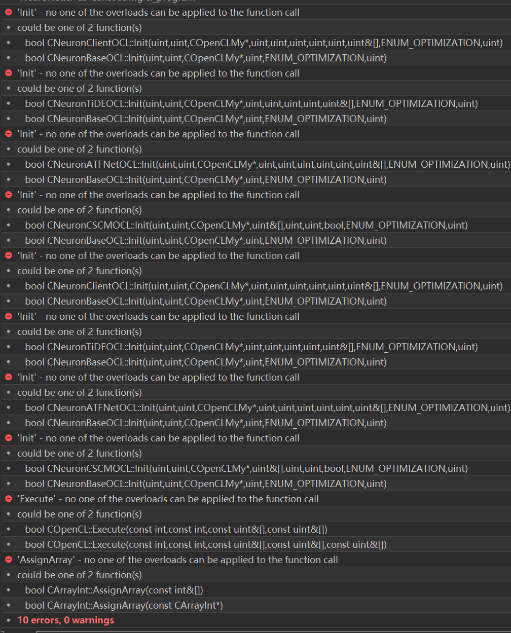
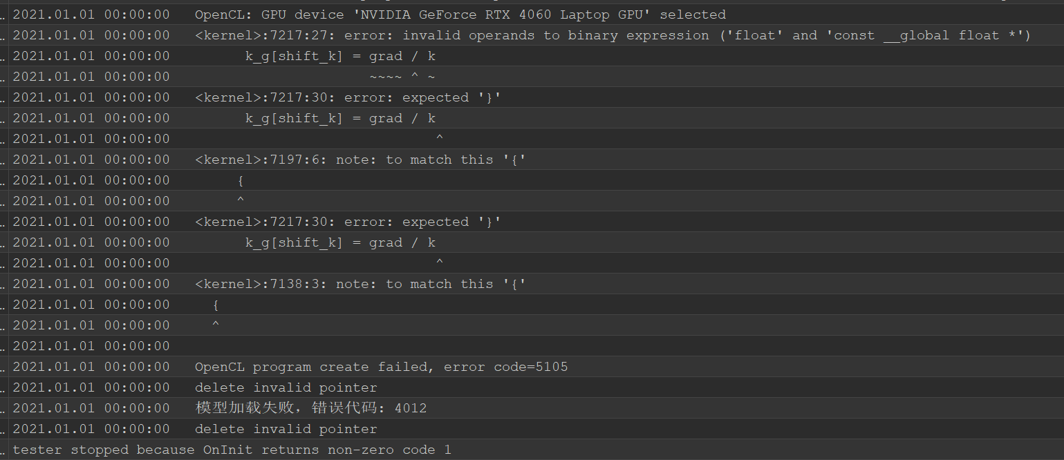 After solving the compilation error, there is a tester error, the whole head is burned, can not figure out where to solve the problem
- Free trading apps
- Over 8,000 signals for copying
- Economic news for exploring financial markets
You agree to website policy and terms of use