Neural Networks in Trading: Market Analysis Using a Pattern Transformer

Introduction

Over the past decade, deep learning (DL) has achieved significant progress across various fields, and these advancements have attracted the attention of researchers in financial markets. Inspired by the success of DLs, many aim to apply it to market trend forecasting and the analysis of complex data interrelationships. A key aspect of such analysis is the representation format of the raw data, which should preserve the inherent relationships and structure of the analyzed instruments. Most existing models operate with homogeneous graphs, limiting their ability to capture the rich semantic information associated with market patterns. Similar to the use of N-grams in natural language processing, frequently occurring market patterns can be leveraged to more precisely identify interconnections and forecast trends.

To address this problem, we decided to adopt certain approaches from the field of chemical element analysis. Much like market patterns, motifs (meaningful subgraphs) frequently occur in molecular structures and can be used to reveal molecular properties. Let's explore the Molformer framework, introduced in the paper "Molformer: Motif-based Transformer on 3D Heterogeneous Molecular Graphs".

The authors of the Molformer method define a novel heterogeneous molecular graph (HMG) as the model's input, comprising nodes at both the atomic and motif levels. This design provides a clean interface for integrating nodes of different levels and prevents the propagation of errors caused by improper semantic segmentation of atoms. Regarding motifs, the authors employ different strategies for different molecule types. For small molecules, the motif vocabulary is determined by functional groups, grounded in chemical domain knowledge. For proteins, composed of sequential amino acids, a reinforcement learning (RL)-based method for intelligent motif mining is introduced to identify the most significant amino acid subsequences.

To align effectively with the HMG, the Molformer framework introduces an equivariant geometric model built on the Transformer architecture. Molformer stands apart from previously considered Transformer-based models in two key aspects. First, it employs heterogeneous Self-Attention (HSA) to capture interactions between nodes of different levels. Second, an Attentive Farthest Point Sampling (AFPS) algorithm is introduced to aggregate node features and obtain a comprehensive representation of the entire molecule.

The authors' paper presents experimental results demonstrating the effectiveness of this approach in addressing challenges within the chemical industry. Let's evaluate the potential of these methods to solve trend forecasting tasks in financial markets.

1. The Molformer Algorithm

Motifs represent frequently occurring substructural patterns and serve as the building blocks of complex molecular structures. They encapsulate a wealth of biochemical characteristics of entire molecules. In the chemical community, a set of standard criteria has been developed for identifying motifs with significant functional capabilities in small molecules. In large protein molecules, motifs correspond to local regions of three-dimensional structures or amino acid sequences common to proteins that influence their function. Each motif typically consists of only a few elements and can describe the connections between secondary structural elements. Based on this property, the authors of the Molformer framework devised a heuristic approach for discovering protein motifs using reinforcement learning (RL). In their work, they propose focusing on motifs composed of four amino acids, which form the smallest polypeptides and possess distinct functional properties in proteins. At this stage, the primary objective is to identify the most effective lexicon 𝓥 from among K quartic amino acid matrices. Since the goal is to find an optimal lexicon for a specific task, it is practically feasible to consider only the existing quartets from downstream datasets rather than all possible combinations.

The learned lexicon 𝓥 is used as templates for motif extraction and for constructing HMGs in downstream tasks. Based on these HMGs, Molformer is then trained. Its effectiveness is treated as the reward r for updating the parameters θ via policy gradients. As a result, the agent can select the optimal lexicon of quartic motifs for the specific task.

Notably, the proposed motif mining process represents a single-step game, as the policy network πθ generates the lexicon 𝓥 only once per iteration. Therefore, the trajectory consists of just one action, and the Molformer outcome, based on the chosen lexicon 𝓥, constitutes part of the overall reward.

The authors of the framework separate motifs and atoms, treating motifs as new nodes for forming the HMG. This disentangles motif-level and atom-level representations, thereby facilitating the model's task of accurately extracting semantic meanings at the motif level.

Similar to the relationships between phrases and individual words in natural language, motifs in molecules carry higher-level semantic meanings than atoms. Consequently, they play a crucial role in defining the functional capabilities of their atomic constituents. The authors of Molformer treat each category of motif as a new node type and construct the HMG as the model's input, such that the HMG contains both motif-level and atom-level nodes. The positions of each motif are represented by a weighted sum of the 3D coordinates of its constituent elements. Analogous to word segmentation, HMGs composed of multi-level nodes prevent error propagation due to improper semantic segmentation by leveraging atomic information to guide molecular representation learning.

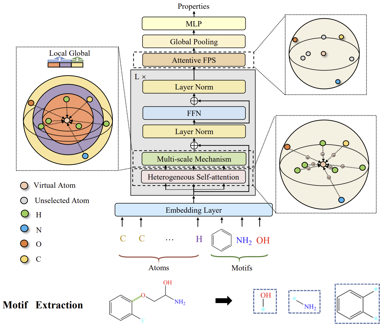
Molformer modifies the Transformer architecture with several new components specifically designed for 3D HMG. Each encoder block consists of HSA, a FeedForward network (FFN), and two-level normalization. This is followed by attentive farthest point sampling (AFPS) to adaptively create a molecular representation, which is then fed into a fully connected predictor for property prediction across a wide range of downstream tasks.

After formulating HMG with N+M nodes at the atom and motif levels, respectively, it is important to provide the model with the ability to differentiate interactions between multi-order nodes. To achieve this, the authors introduce a function φ(i,j)→Z, which defines relationships between any two nodes in three types: atom-atom, atom-motif, and motif-motif. A learnable scalar bφ(i,j) is then introduced to adaptively handle all nodes according to their hierarchical relationships within the HMG.

Furthermore, the authors consider the use of three-dimensional molecular geometry. Since robustness to global changes such as 3D translations and rotations is a foundational principle of molecular representation learning, they aim to ensure roto-translational invariance by applying a convolution operation to the pairwise distance matrix 𝑫.

Moreover, the use of local context has proven important in sparse 3D spaces. However, it has been observed that Self-Attention effectively captures global data patterns but tends to overlook local context. Based on this observation, the authors impose a distance-based constraint on Self-Attention to extract multi-scale patterns from both local and global contexts. For this purpose, a multi-scale methodology was developed for reliably capturing details. Specifically, nodes outside a certain distance threshold τs at each scale s are masked out. Then, features extracted at different scales are combined into a multi-scale representation and fed into the FFN.

The original visualization of the Molformer framework is provided below.

2. Implementation in MQL5

After reviewing the theoretical aspects of the Molformer method, we now move on to the practical part of the article, where we implement our interpretation of the proposed approaches using MQL5. As in our previous work, we will divide the entire process of implementing the framework into separate modules that perform recurring operations.

2.1 Attention pooling

To begin, we will isolate the dependency-based pooling algorithm proposed by the authors of the R-MAT method into a standalone class.

Do not be surprised that we are starting the implementation of the Molformer framework by incorporating an approach from the R-MAT method. Both methods were proposed to address similar challenges in the chemical industry. In our view, there are some intersections between them that we will use. The dependency-based pooling algorithm is one of these intersections.

We will organize the processes of this algorithm into the class CNeuronMHAttentionPooling, the structure of which is presented below.

class CNeuronMHAttentionPooling  :  public   CNeuronBaseOCL
  {
protected:
   uint              iWindow;
   uint              iHeads;
   uint              iUnits;
   CLayer            cNeurons;
   //---
   virtual bool      feedForward(CNeuronBaseOCL *NeuronOCL) override;
   virtual bool      calcInputGradients(CNeuronBaseOCL *NeuronOCL) override;
   virtual bool      updateInputWeights(CNeuronBaseOCL *NeuronOCL) override;

public:
                     CNeuronMHAttentionPooling(void) {};
                    ~CNeuronMHAttentionPooling(void) {};
   //---
   virtual bool      Init(uint numOutputs, uint myIndex, COpenCLMy *open_cl,
                          uint window, uint units_count, uint heads,
                          ENUM_OPTIMIZATION optimization_type, uint batch);
   //---
   virtual int       Type(void) override   const   {  return defNeuronMHAttentionPooling; }
   //---
   virtual bool      Save(int const file_handle) override;
   virtual bool      Load(int const file_handle) override;
   //---
   virtual bool      WeightsUpdate(CNeuronBaseOCL *source, float tau) override;
   virtual void      SetOpenCL(COpenCLMy *obj) override;
  };

In this class, we declare three internal variables and one dynamic array in which we will store pointers to internal objects in the sequence they are called. The array itself is declared statically, allowing us to leave the constructor and destructor of the class empty. The initialization of all inherited and newly declared objects is performed in the Init method, which takes as parameters constants that unambiguously define the architecture of the created object.

bool CNeuronMHAttentionPooling::Init(uint numOutputs, uint myIndex, COpenCLMy *open_cl,
                                     uint window, uint units_count, uint heads,
                                     ENUM_OPTIMIZATION optimization_type, uint batch)
  {
   if(!CNeuronBaseOCL::Init(numOutputs, myIndex, open_cl, window * units_count, optimization_type, batch))
      return false;

In the body of the object initialization method, we first call the parent class method of the same name, where part of the necessary controls and the initialization algorithm of inherited objects have already been implemented. Afterward, we store the constants received from the external program into the internal variables.

   iWindow = window;
   iUnits = units_count;
   iHeads = heads;

We prepare our dynamic array.

   cNeurons.Clear();
   cNeurons.SetOpenCL(OpenCL);

And then we start creating a structure of nested objects. Here we create a two-layer MLP, in which we use the hyperbolic tangent to create nonlinearity between neural layers.

   int idx = 0;
   CNeuronConvOCL *conv = new CNeuronConvOCL();
   if(!conv ||
      !conv.Init(0, idx, OpenCL, iWindow*iHeads, iWindow*iHeads, 4*iWindow, iUnits, 1, optimization, iBatch) ||
      !cNeurons.Add(conv)
     )
      return false;
   idx++;
   conv.SetActivationFunction(TANH);
   conv = new CNeuronConvOCL();
   if(!conv ||
      !conv.Init(0, idx, OpenCL, 4*iWindow, 4*iWindow, iHeads, iUnits, 1, optimization, iBatch) ||
      !cNeurons.Add(conv)
     )
      return false;

The output of the MLP is normalized by the Softmax function in terms of individual elements of the sequence.

   idx++;
   conv.SetActivationFunction(None);
   CNeuronSoftMaxOCL *softmax = new CNeuronSoftMaxOCL();
   if(!softmax ||
      !softmax.Init(0, idx, OpenCL, iHeads * iUnits, optimization, iBatch) ||
      !cNeurons.Add(softmax)
     )
      return false;
   softmax.SetHeads(iUnits);
//---
   return true;
  }

We conclude the method by returning a boolean result indicating the success of the operations to the calling program.

It is important to note that in this case, we do not perform any pointer substitution for data buffers. This is because the objects we create only generate intermediate data. The actual result of the created object is formed by multiplying the normalized outputs of the created MLP by the input data tensor. The results of this operation are then stored in the corresponding buffer inherited from the parent class. A similar approach applies to the error gradient buffer.

Once the initialization method of the class is complete, we move on to constructing the forward pass algorithm in the feedForward method.

bool CNeuronMHAttentionPooling::feedForward(CNeuronBaseOCL *NeuronOCL)
  {
   CNeuronBaseOCL *current = NULL;
   CObject *prev = NeuronOCL;

In the method parameters, we receive a pointer to the source data object. In the body of the method, we declare two local variables for temporary storage of pointers to objects. We pass a pointer to the source data object to one of them.

Next we organize a loop through the internal MLP objects with a sequential call to the same-name methods of the internal model.

   for(int i = 0; i < cNeurons.Total(); i++)
     {
      current = cNeurons[i];
      if(!current ||
         !current.FeedForward(prev)
        )
         return false;
      prev = current;;
     }

After completing all iterations of the loop, we obtain the attention head influence coefficients for each individual element in the sequence. Now, as previously mentioned, we need to compute the weighted average of the attention heads in the input data by multiplying the obtained coefficients with the input data tensor. The result of this tensor multiplication is stored in the result buffer of our object.

   if(!MatMul(current.getOutput(), NeuronOCL.getOutput(), Output,
                                      1, iHeads, iWindow, iUnits))
      return false;
//---
   return true;
  }

Finally, we return the boolean result of the operations to the calling program, concluding the method.

I suggest leaving the backpropagation methods of this class for independent study. The full code of this class and all its methods can be found in the attachment.

2.2 Pattern Extraction

In the next stage of our work, we will create the pattern extraction object. As mentioned in the theoretical section, pattern embeddings are added to the input data tensor before being passed to the model. However, we will approach this differently: we will feed the model a standard dataset as input, and the pattern extraction and concatenation of their embeddings with the input data tensor will be performed within the model itself.

It is important to note that each pattern embedding added to the input data must have the dimensionality of a single sequence element and lie within the same subspace The first issue will be addressed through architectural decisions. The second issue we will attempt to resolve during the training of the pattern embeddings.

To accomplish these tasks, we will create a new class CNeuronMotifs. Its structure is presented below.

class CNeuronMotifs    :  public CNeuronBaseOCL
  {
protected:
   CNeuronConvOCL    cMotifs;
   //---
   virtual bool      feedForward(CNeuronBaseOCL *NeuronOCL) override;
   virtual bool      calcInputGradients(CNeuronBaseOCL *NeuronOCL) override;
   virtual bool      updateInputWeights(CNeuronBaseOCL *NeuronOCL) override;

public:
                     CNeuronMotifs(void) {};
                    ~CNeuronMotifs(void) {};
   //---
   virtual bool      Init(uint numOutputs, uint myIndex, COpenCLMy *open_cl,
                          uint dimension, uint window, uint step, uint units_count,
                          ENUM_OPTIMIZATION optimization_type, uint batch);
   //---
   virtual int       Type(void) override   const   {  return defNeuronMotifs; }
   //---
   virtual bool      Save(int const file_handle) override;
   virtual bool      Load(int const file_handle) override;
   //---
   virtual bool      WeightsUpdate(CNeuronBaseOCL *source, float tau) override;
   virtual void      SetOpenCL(COpenCLMy *obj) override;
   //---
   virtual void      SetActivationFunction(ENUM_ACTIVATION value) override;
  };

In this class, we declare only one internal convolutional layer, which will be responsible for performing the pattern embedding functionality. However, it is noteworthy that we override the method for specifying the activation function. Interestingly, this method has not been overridden in any of our previous implementations. In this case, it is done to synchronize the activation function of the internal layer with that of the object itself.

void CNeuronMotifs::SetActivationFunction(ENUM_ACTIVATION value)
  {
   CNeuronBaseOCL::SetActivationFunction(value);
   cMotifs.SetActivationFunction(activation);
  }

We initialize the declared convolutional layer, as well as all inherited objects, in the Init method. In the parameters of this method, we pass constants that allow us to uniquely determine the architecture of the object being created.

bool CNeuronMotifs::Init(uint numOutputs, uint myIndex, COpenCLMy *open_cl,
                         uint dimension, uint window, uint step, uint units_count,
                         ENUM_OPTIMIZATION optimization_type, uint batch
                        )
  {
   uint inputs = (units_count * step + (window - step)) * dimension;
   uint motifs = units_count * dimension;

However, unlike similar methods we considered earlier, in this case we do not have sufficient data to directly call the method of the same name from the parent class. This is primarily due to the size of the result buffer. As mentioned above, the output we expect is a concatenated tensor of the input data and the pattern embeddings. Therefore, we will first determine the sizes of the input data tensor and the pattern embedding tensor based on the available data, and only then call the initialization method of the parent class, passing in the sum of the determined sizes.

   if(!CNeuronBaseOCL::Init(numOutputs, myIndex, open_cl, inputs + motifs, optimization_type, batch))
      return false;

The next step is to initialize the internal pattern embedding convolutional layer according to the parameters received from the external program.

   if(!cMotifs.Init(0, 0, OpenCL, dimension * window, dimension * step, dimension, units_count,
                                                                           1, optimization, iBatch))
      return false;

Note that the size of the returned embeddings is equal to the dimension of the input data.

We forcibly cancel the activation function using the method overridden above.

   SetActivationFunction(None);
//---
   return true;
  }

After that, we complete the method by passing the bool result of the operations to the calling program.

The initialization of the object is followed by the construction of feed-forward pass processes, which we implement in the feedForward method. Here everything is quite straightforward.

bool CNeuronMotifs::feedForward(CNeuronBaseOCL *NeuronOCL)
  {
   if(!NeuronOCL)
      return false;

It takes as a parameter a pointer to the input data object, and the first step is to verify the validity of this pointer. After that, we synchronize the activation functions of the input data layer and the current object.

   if(NeuronOCL.Activation() != activation)
      SetActivationFunction((ENUM_ACTIVATION)NeuronOCL.Activation());

This operation will allow us to synchronize the output area of the embedding layer with the input data.

And only after carrying out the preparatory work we carry out a feed-forward pass of the inner layer.

   if(!cMotifs.FeedForward(NeuronOCL))
      return false;

Then we concatenate the tensor of the obtained embeddings with the input data.

   if(!Concat(NeuronOCL.getOutput(), cMotifs.getOutput(), Output, NeuronOCL.Neurons(), cMotifs.Neurons(), 1))
      return false;
//---
   return true;
  }

We write the concatenated tensor to the result buffer inherited from the parent class and conclude the method by returning a boolean result indicating the success of the operations to the calling program.

Next, we move on to working on backpropagation methods. And as you might have guessed, their algorithm is just as simple. For example, in the error gradient distribution method calcInputGradients, we perform only one operation of deconcatenation of the error gradient buffer inherited from the parent class, distributing the values between the input data object and the internal layer.

bool CNeuronMotifs::calcInputGradients(CNeuronBaseOCL *NeuronOCL)
  {
   if(!NeuronOCL)
      return false;
   if(!DeConcat(NeuronOCL.getGradient(),cMotifs.getGradient(),Gradient,NeuronOCL.Neurons(),cMotifs.Neurons(),1))
      return false;
//---
   return true;
  }

However, this apparent simplicity requires a few clarifications. First, we do not adjust the error gradient passed to the input data and the internal layer by the derivative of the activation function of the corresponding objects. In this case, such an operation is redundant. This is achieved by synchronizing the activation function pointer of our object, the internal layer, and the input data, which we established when designing the feed-forward pass method. This simple operation allowed us to obtain the error gradient, already adjusted by the derivative of the correct activation function, at the level of the object results. Consequently, we perform the deconcatenation on the already adjusted error gradient.

The second point to note is that we do not pass the error gradient from the internal pattern extraction layer to the input data. Interestingly, the reason for this is the nature of our task: pattern extraction from input data. Our goal is to identify the significant patterns, not to "fit" the input data to the desired patterns. However, as can be easily seen, the input data still receives its own error gradient through the direct data flow.

The full code of this class and all its methods can be found in the attachment.

2.3 Multi-Scale Attention

Another "building block" we need to create is the multi-scale attention object. I must say that here we made perhaps the most significant deviation from the original Molformer algorithm. The authors of the framework implemented a masking mechanism that excluded objects located beyond a certain distance from the target. Thereby, they focused attention only within a defined area.

In our implementation, however, we took a different approach. First, instead of the proposed attention mechanism, we used the Relative Self-Attention method discussed in the previous article, which analyzes not only positional offsets but also contextual information. Second, to adjust the attention scale, we increase the size of a single analyzed element to cover two, three, and four elements of the original sequence. This can be likened to analyzing a higher timeframe chart. The implementation of our solution is presented in the CNeuronMultiScaleAttention class. The structure of the new class is shown below.

class CNeuronMultiScaleAttention :  public CNeuronBaseOCL
  {
protected:
   uint              iWindow;
   uint              iUnits;
   //---
   CNeuronBaseOCL    cWideInputs;
   CNeuronRelativeSelfAttention  cAttentions[4];
   CNeuronBaseOCL    cConcatAttentions;
   CNeuronMHAttentionPooling cPooling;
   //---
   virtual bool      feedForward(CNeuronBaseOCL *NeuronOCL) override;
   virtual bool      calcInputGradients(CNeuronBaseOCL *NeuronOCL) override;
   virtual bool      updateInputWeights(CNeuronBaseOCL *NeuronOCL) override;

public:
                     CNeuronMultiScaleAttention(void) {};
                    ~CNeuronMultiScaleAttention(void) {};
   //---
   virtual bool      Init(uint numOutputs, uint myIndex, COpenCLMy *open_cl,
                          uint window, uint window_key, uint units_count, uint heads,
                          ENUM_OPTIMIZATION optimization_type, uint batch);
   //---
   virtual int       Type(void) override   const   {  return defNeuronMultiScaleAttention; }
   //---
   virtual bool      Save(int const file_handle) override;
   virtual bool      Load(int const file_handle) override;
   //---
   virtual bool      WeightsUpdate(CNeuronBaseOCL *source, float tau) override;
   virtual void      SetOpenCL(COpenCLMy *obj) override;
  };

Here we explicitly define the number of scales by declaring a fixed array of relative attention objects. In addition, the class structure declares 3 more objects, the purpose of which we will become familiar with during the implementation of the class methods.

We declare all internal objects as static and thus we can leave the class constructor and destructor empty. The initialization of these declared and inherited objects is performed in the Init method.

bool CNeuronMultiScaleAttention::Init(uint numOutputs, uint myIndex,
                                      COpenCLMy *open_cl, uint window,
                                      uint window_key, uint units_count,
                                      uint heads,
                                      ENUM_OPTIMIZATION optimization_type,
                                      uint batch)
  {
   if(!CNeuronBaseOCL::Init(numOutputs, myIndex, open_cl, window * units_count, optimization_type, batch))
      return false;

In the method parameters, as usual, we receive constants that uniquely define the architecture of the created object. Within the body of the method, we immediately call the identically named method of the parent class. I believe it is unnecessary to repeat that this method already contains the necessary checks and initialization algorithms for inherited objects.

After the successful execution of the parent class method, we store some constants in internal variables.

   iWindow = window;
   iUnits = units_count;

Before initializing the newly declared objects, it is important to note that at this stage we do not know the size of the input data tensor. Moreover, we do not know whether its dimensions are compatible with our analysis scales. In fact, the input tensor we receive might not even be a multiple of our scales. However, the tensors fed into the large-scale attention objects need to be of the correct size. To meet this requirement, we will create an internal object into which we will copy the input data, adding zero values to fill in any missing elements. But first, we will determine the required buffer size as the maximum of the nearest larger multiples of our scales.

   uint units1 = (iUnits + 1) / 2;
   uint units2 = (iUnits + 2) / 3;
   uint units3 = (iUnits + 3) / 4;
   uint wide = MathMax(MathMax(iUnits, units1 * 2), MathMax(units2 * 3, units3 * 4));

Then we initialize the object to copy the input data of the required size.

   int idx = 0;
   if(!cWideInputs.Init(0, idx, OpenCL, wide * iWindow, optimization, iBatch))
      return false;
   CBufferFloat *temp = cWideInputs.getOutput();
   if(!temp || !temp.Fill(0))
      return false;

We fill the result buffer of this layer with zero values.

In the next step, we initialize internal attention objects of different scales while maintaining other parameters.

   idx++;
   if(!cAttentions[0].Init(0, idx, OpenCL, iWindow, window_key, iUnits, heads, optimization, iBatch))
      return false;
   idx++;
   if(!cAttentions[1].Init(0, idx, OpenCL, 2 * iWindow, window_key, units1, heads, optimization, iBatch))
      return false;
   idx++;
   if(!cAttentions[2].Init(0, idx, OpenCL, 3 * iWindow, window_key, units2, heads, optimization, iBatch))
      return false;
   idx++;
   if(!cAttentions[3].Init(0, idx, OpenCL, 4 * iWindow, window_key, units3, heads, optimization, iBatch))
      return false;

It should be noted here that despite the different scales of the objects of attention, we expect to obtain tensors of comparable sizes at the output. This is because, in essence, they all use a single source of initial data. Therefore, to concatenate the attention results, we will declare the object to be 4 times larger than the original data.

   idx++;
   if(!cConcatAttentions.Init(0, idx, OpenCL, 4 * iWindow * iUnits, optimization, iBatch))
      return false;

To average the attention results, we will use the dependency-based pooling class created above.

   idx++;
   if(!cPooling.Init(0, idx, OpenCL, iWindow, iUnits, 4, optimization, iBatch))
      return false;

Then we substitute the pointers of the result buffers and error gradients of the created object with pointers of the corresponding buffers of the pooling layer.

   SetActivationFunction(None);
   if(!SetOutput(cPooling.getOutput()) ||
      !SetGradient(cPooling.getGradient()))
      return false;
//---
   return true;
  }

At the end of the method, we pass the operation results to the calling program.

Note that in this class we have not organized objects to implement the residual connections, which we used in the previously discussed attention blocks. This is because the internal relative attention blocks we use already incorporate residual connections. As a result, the averaging of attention outcomes already accounts for these residual connections. Adding further operations would be redundant.

After initializing the object, we move on to constructing the feed-forward pass processes, which we will implement in the feedForward method.

bool CNeuronMultiScaleAttention::feedForward(CNeuronBaseOCL *NeuronOCL)
  {
//--- Attention
   if(!cAttentions[0].FeedForward(NeuronOCL))
      return false;

In the parameters of the feedForward method, as usual, we receive a pointer to the input data object, which we immediately pass to the method of the same name in the internal single-scale attention layer. In the method of the internal object, in addition to the core operations, we also check the validity of the received pointer. Consequently, after the successful execution of the internal class method operations, we can safely use the pointer obtained from the external program. In the next step, we transfer the input data into the buffer of the corresponding internal layer. After this, we synchronize the activation functions.

   if(!Concat(NeuronOCL.getOutput(), NeuronOCL.getOutput(), cWideInputs.getOutput(), iWindow, 0, iUnits))
      return false;
   if(cWideInputs.Activation() != NeuronOCL.Activation())
      cWideInputs.SetActivationFunction((ENUM_ACTIVATION)NeuronOCL.Activation());

It is important to note that, in this case, we use a concatenation method for copying the input data, in which we specify the pointer to the result buffer of the input data object twice. For the first buffer, we indicate the window size of the input data, and for the second it is "0". Clearly, with these parameter settings, we will obtain a copy of the input data in the specified result buffer. At the same time, no explicit operation of adding zero values for missing data, which we discussed during object initialization, is performed.

However, the addition of zero values occurs implicitly. During the initialization of the internal input data object, we filled its result buffer with zero values. During training and operation, we expect to receive input data tensors of the same size. Consequently, each time we copy the input data, we will overwrite the same elements, while the remaining ones will remain filled with zeros.

After forming the expanded input data object, we organize a loop to perform multi-scale attention operations. In this loop, we will sequentially call the feed-forward pass methods of the larger-scale attention objects, passing them the pointer to the expanded input data object.

//--- Multi scale attentions
   for(int i = 1; i < 4; i++)
      if(!cAttentions[i].FeedForward(cWideInputs.AsObject()))
         return false;

We concatenate the results of attention of all scales into a single tensor. Despite the difference in the scale of the analyzed data, the output produces comparable tensors, and each element of the original sequence remains in its place. Therefore, we perform the concatenation of tensors in the context of the elements of the original sequence.

//--- Concatenate Multi-Scale Attentions
   if(!Concat(cAttentions[0].getOutput(), cAttentions[1].getOutput(), cAttentions[2].getOutput(),
              cAttentions[3].getOutput(), cConcatAttentions.getOutput(), 
              iWindow, iWindow, iWindow, iWindow, iUnits))
      return false;

And then, in the same way, in terms of the elements of the original sequence, we perform weighted pooling of the results of multi-scale attention, taking into account dependencies.

//--- Attention pooling
   if(!cPooling.FeedForward(cConcatAttentions.AsObject()))
      return false;
//---
   return true;
  }

Before concluding the method, we return a boolean value indicating the success or failure of the initialization to the caller.

As a reminder, during the initialization phase of the object, we replaced the pointers to the result buffers and error gradient buffers. Therefore, the pooling results are directly placed into the buffers used for communication between the neural network layers of the model. Consequently, we omit the redundant data copying operation.

I suggest leaving the backpropagation methods of this class for independent study. The complete code for this class and all of its methods is provided in the attached files.

2.4 Constructing the Molformer Framework

A substantial amount of work has been done above to build the individual components of the Molformer framework. Now, it’s time to assemble these individual components into the complete architecture of the framework. For this purpose, we will create a new CNeuronMolformer class. In this case, we will use CNeuronRMAT as the parent class, which implements the mechanism of the simplest linear model. The structure of the new class is shown below.

class CNeuronMolformer  :  public CNeuronRMAT
  {
public:
                     CNeuronMolformer(void) {};
                    ~CNeuronMolformer(void) {};
   //---
   virtual bool      Init(uint numOutputs, uint myIndex, COpenCLMy *open_cl,
                          uint window, uint window_key,
                          uint units_count, uint heads, uint layers,
                          uint motif_window, uint motif_step,
                          ENUM_OPTIMIZATION optimization_type, uint batch); //Molformer
   //---
   virtual int       Type(void) override   const   {  return defNeuronMolformer; }
  };

Note that, unlike the previously implemented components, here we override only the initialization method of the new class Init. This was made possible thanks to the linear structure organized in the parent class. Now, it is sufficient to populate the dynamic array, inherited from the parent class, with the required sequence of objects. The entire interaction algorithm between these components is already constructed within the methods of the parent class.

In the parameters of this sole overridden method, we receive a series of constants that allow us to unambiguously interpret the architecture of the created object as intended by the user.

bool CNeuronMolformer::Init(uint numOutputs, uint myIndex, COpenCLMy *open_cl,
                            uint window, uint window_key, uint units_count,
                            uint heads, uint layers,
                            uint motif_window, uint motif_step,
                            ENUM_OPTIMIZATION optimization_type, uint batch)
  {
   if(!CNeuronBaseOCL::Init(numOutputs, myIndex, open_cl, window * units_count, optimization_type, batch))
      return false;

In the body of the method, we immediately call the method of the base class of the fully connected neural layer.

It's important to note that we call the method of the base neural layer class, rather than that of the direct parent object. In the body of the method, we need to create a completely new architecture. So, we will not recreate the architectural solutions of the parent class.

The next step is to prepare a dynamic array, in which we will store pointers to the objects being created.

   cLayers.Clear();
   cLayers.SetOpenCL(OpenCL);

Let's now move on to the operations related to the creation and initialization of the required objects. Here we first create and initialize the pattern extraction object. To a dynamic array, we add a pointer to the new object.

   int idx = 0;
   CNeuronMotifs *motif = new CNeuronMotifs();
   uint motif_units = units_count - MathMax(motif_window - motif_step, 0);
   motif_units = (motif_units + motif_step - 1) / motif_step;
   if(!motif ||
      !motif.Init(0, idx, OpenCL, window, motif_window, motif_step, motif_units, optimization, iBatch) ||
      !cLayers.Add(motif)
     )
      return false;

Then we create local variables for temporary storage of pointers to objects and run a loop, which will create internal layers of the Encoder. The number of the internal layers is by a constant in the method parameters.

   idx++;
   CNeuronMultiScaleAttention *msat = NULL;
   CResidualConv *ff = NULL;
   uint units_total = units_count + motif_units;
   for(uint i = 0; i < layers; i++)
     {
      //--- Attention
      msat = new CNeuronMultiScaleAttention();
      if(!msat ||
         !msat.Init(0, idx, OpenCL, window, window_key, units_total, heads, optimization, iBatch) ||
         !cLayers.Add(msat)
        )
         return false;
      idx++;

In the loop body, we first create and initialize the multiscale attention object. And then we add a convolutional block with residual connection.

      //--- FeedForward
      ff = new CResidualConv();
      if(!ff ||
         !ff.Init(0, idx, OpenCL, window, window, units_total, optimization, iBatch) ||
         !cLayers.Add(ff)
        )
         return false;
      idx++;
     }

We add pointers to the created objects to the dynamic array of internal objects.

Next, note that at the output of the multiscale attention block, we obtain a concatenated tensor of the input data and pattern embeddings, enriched with information about internal dependencies. However, at the output of the class, we need to return a tensor of enriched input data. Instead of simply "discarding" the pattern embeddings, we will use a scaling function for the data within individual unit sequences. To do this, we first transpose the results of the previous layer.

//--- Out
   CNeuronTransposeOCL *transp = new CNeuronTransposeOCL();
   if(!transp ||
      !transp.Init(0, idx, OpenCL, units_total, window, optimization, iBatch) ||
      !cLayers.Add(transp)
     )
      return false;
   idx++;

Then we add a convolutional layer that will perform the functionality of scaling individual unitary sequences.

   CNeuronConvOCL *conv = new CNeuronConvOCL();
   if(!conv ||
      !conv.Init(0, idx, OpenCL, units_total, units_total, units_count, window, 1, optimization, iBatch) ||
      !cLayers.Add(conv)
     )
      return false;
   idx++;

Reset the output to the original data representation.

   idx++;
   transp = new CNeuronTransposeOCL();
   if(!transp ||
      !transp.Init(0, idx, OpenCL, window, units_count, optimization, iBatch) ||
      !cLayers.Add(transp)
     )
      return false;

After that, we just need to substitute the pointers to the data buffers and return the logical result of the operations to the calling program.

   if(!SetOutput(transp.getOutput()) ||
      !SetGradient(transp.getGradient()))
     return false;
//---
   return true;
  }

With this, we conclude our discussion of the Molder framework classes. You can find the complete source code for all presented classes and their methods in the attachment. The attachment also contains complete code for all programs used in the article. Please note that we are using interaction and training programs from earlier articles. Some minor changes were made to the architecture of the Environment State Encoder, which I encourage you to explore independently. You can find a full description of the architecture of the trainable models in the attachment. We now proceed to the final stage of our work - training the models and testing the results.

3. Testing

In this article, we implemented the Molformer framework in MQL5 and are now moving to the final stage – training the models and evaluating the trained Actor behavior policy. We follow the training algorithm described in previous works, and we simultaneously train three models: the State Encoder, Actor, and Critic. The Encoder analyzes the market situation, the Actor executes trades based on the learned policy, and the Critic evaluates the Actor's actions and provides guidance for refining the behavior policy.

The training is conducted using real historical EURUSD data on the H1 timeframe for the entire year 2023, with standard parameters for the analyzed indicators.

The training process is iterative. It includes periodic updates of the training dataset.

To verify the effectiveness of the trained policy, we use historical data for January 2024. The test results are presented below.

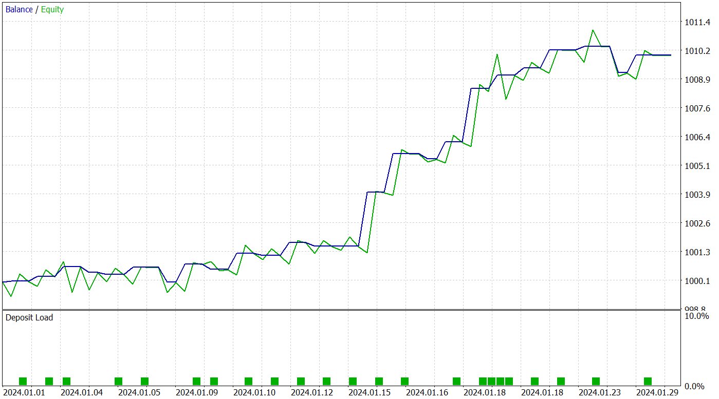
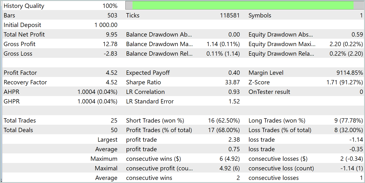
The trained model executed 25 trades during the test period, of which 17 closed with a profit. This represents 68% of the total. Moreover, the average and maximum profitable trades are twice as large as the corresponding loss-making trades.

The potential of the proposed model is also confirmed by the equity curve, which demonstrates a clear upward trend. However, the short testing period and limited number of trades suggest that this result only indicates potential.

Conclusion

The Molformer method represents a significant advancement in the field of market data analysis and forecasting. By utilizing heterogeneous market graphs, which include both individual assets and their combinations in the form of market patterns, the model is able to consider more complex relationships and data structures, which significantly improves the accuracy of forecasting future price movements.

In the practical part of the article, we implemented our vision of Molformer approaches using MQL5. We integrated the proposed solutions into the model and trained it on real historical data. As a result, we have created a model capable of generalizing the acquired knowledge to new market situations and generating profit. This is confirmed by the testing results. We believe that the proposed approach can become a foundation for further research and applications in the field of financial analysis, providing traders and analysts with new tools for making informed decisions in conditions of uncertainty.

References

• Molformer: Motif-based Transformer on 3D Heterogeneous Molecular Graphs
• Other articles from this series

Programs used in the article

#	Name	Type	Description
1	Research.mq5	Expert Advisor	EA for collecting examples
2	ResearchRealORL.mq5	Expert Advisor	EA for collecting examples using the Real-ORL method
3	Study.mq5	Expert Advisor	Model training EA
4	Test.mq5	Expert Advisor	Model testing EA
5	Trajectory.mqh	Class library	System state description structure
6	NeuroNet.mqh	Class library	A library of classes for creating a neural network
7	NeuroNet.cl	Library	OpenCL program code library