
Neural Networks in Trading: Dual-Attention-Based Trend Prediction Model

Introduction
The price of a financial instrument represents a highly volatile time series influenced by numerous factors, including interest rates, inflation, monetary policy, and investor sentiment. Modeling the relationship between the price of a financial instrument and these factors, as well as forecasting their dynamics, is a significant challenge for researchers and investors.
A vast body of research has been dedicated to the prediction and analysis of financial time series. Traditional statistical methods often assume that time series are generated by linear processes, which limits their effectiveness in non-linear forecasting. Machine learning and deep learning methods have demonstrated greater success in modeling financial time series due to their ability to capture non-linear relationships. Many studies have focused on extracting features at specific time points and using them for modeling and prediction. However, such approaches often overlook data interactions and the short-term continuity of fluctuations.
To address these limitations, the study "A Dual-Attention-Based Stock Price Trend Prediction Model With Dual Features" proposes a dual-feature extraction method. This method leverages both individual time points and multiple temporal intervals. It integrates short-term market features with long-term temporal features to enhance prediction accuracy. The proposed model is based on an Encoder-Decoder architecture and employs attention mechanisms in both the Encoder and Decoder stages, enabling the identification of the most relevant features in long time series.
This research introduces a new Trend Prediction Model (TPM) designed to predict stock price trends by using dual-feature extraction and dual-attention mechanisms. The TPM aims to forecast both the direction and duration of stock price movements. The key contributions of the proposed approach are as follows:
- A novel dual-feature extraction method based on different time ranges, which effectively extracts important market information and optimizes forecasting results. TPM uses piecewise linear regression and a convolutional neural network to extract long-term and short-term market features from financial time series, respectively. The representation of market information through dual features significantly enhances the model's predictive performance.
- Stock price Trend Prediction Model (TPM) using the Encoder-Decoder structure and dual-attention mechanism. By adding attention mechanisms in both the Encoder and Decoder stages, TPM adaptively selects the most relevant short-term market features and combines them with long-term temporal features to improve forecasting accuracy.
1. TPM Algorithm
Upon analyzing existing time series forecasting methods, the authors of TPM came to the following conclusions:
- Univariate financial time series lack sufficient information for confident prediction of future price movements.
- Traditional feature extraction methods are limited in capturing complex market behaviors.
- Time series analysis using a single neural network is incomplete.
The TPM method addresses these issues by employing dual-feature extraction and dual-attention mechanisms. The proposed algorithm consists of two phases. First, piecewise linear regression method is used to segment the financial time series and extract historical long-term temporal features based on subsequences with varying time intervals. Short-term spatial market features are extracted from individual time points using a convolutional neural network.
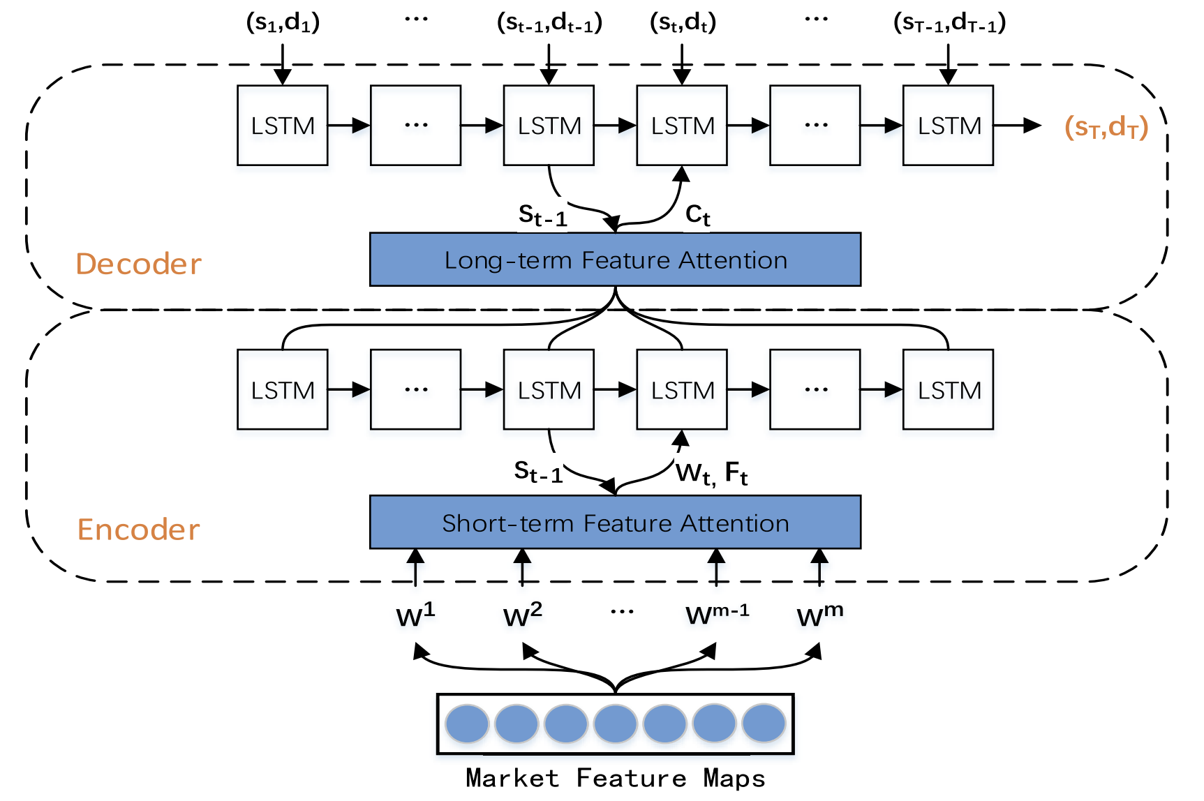
Then, during the second TPM phase, the previously extracted dual features are analyzed by the trend prediction model based on dual-attention mechanisms. The proposed model is built on the Encoder-Decoder architecture.
The encoder is based on a recurrent LSTM block with the addition of an attention mechanism that is used to adaptively extract the most relevant short-term market features.
The decoder is also built using an LSTM block and an attention mechanism that selects and decodes the most relevant combined features to predict the stock price trend.
Since the information provided by a one-dimensional financial time series is insufficient, it is difficult to model and forecast the trend of stock prices based on such data. TPM method authors use basic market data for analysis, such as bar opening and closing prices, maximum and minimum prices, and volume, transforming them into a series of technical indicators.
Given the continuous changes in data, TPM extracts long-term temporal features using piecewise linear regression (PLR). The PLR method smooths out short-term fluctuation noise, reduces data dimensionality and improves computational performance.
The segmentation of a time series depends on the maximum error threshold δ. Taking CSI 300 data as an example, the authors of the method use PLR to segment its historical closing price. With δ equal to 2.0, the time series can be divided into 16 subsequences. However, if the threshold value δ equals 4.0, the same time series can be segmented into only 4 subsequences. Therefore, as the threshold value increases, more data fluctuations are ignored and fewer subsequences are formed. The threshold value affects the reliability of the features of the historical time series. Each subsequence represents a fluctuation in the data over a given period of time. Slope sm and duration dm of each subsequence being generated as long-term temporal features for trend prediction.
Considering the interaction of different data at the same point in time, short-term spatial market features of each time step are extracted using a convolutional neural network (CNN). A market matrix is constructed for the analyzed financial time series. In the market matrix, each row represents one dimension of the analyzed data, and the number of rows is n. Then each column represents one time point. Since CNN preserves the neighborhood relationships and spatial localization of the original data, it can capture the nonlinear relationship between the market matrix and the stock trend. This results in spatial features for short-term historical time series.
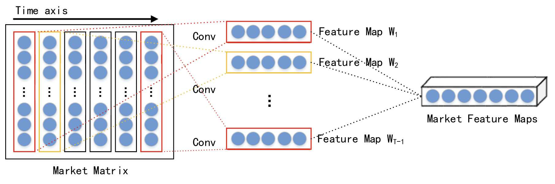
In their work, the authors employ convolutional layers of varying kernel sizes, such as 1 × 3 to 1 × 5, to extract abstract, multi-level spatial market features. The ReLU function is chosen as the non-linear activation function.
Following the convolutional layers, a max pooling layer is applied. This reduces the dimensions of the feature maps and helps prevent overfitting.
The outputs from multiple convolutional and max pooling layers are then passed to a projection layer for further processing.
As mentioned earlier, the extracted short-term and long-term features are processed within the Encoder-Decoder architecture. In this structure, the Encoder compresses the input information into a fixed-size vector, and the Decoder processes these vectors to produce the final output. However, when the input data is extensive, the Encoder may struggle to effectively capture all relevant information, leading to a decline in model performance. The attention mechanism addresses this limitation by decoding the hidden states of the relevant neurons.
It is important to note that the Decoder with an attention mechanism lacks the capability to explicitly select the most relevant input features. To overcome this, the authors of the TPM method add attention mechanisms in both the Encoder and Decoder stages.
The second phase of the TPM algorithm is based on a dual attention mechanism. The Encoder-Decoder structure is divided into two stages. At the first stage the Encoder, which is based on LSTM with the attention mechanism, analyzes short-term spatial market features extracted using CNN. The corresponding short-term features at each time point are selected adaptively and encoded into vectors.
In the second stage, the encoded vectors and long-term temporal features extracted usingPLR are fed to an LSTM-based Decoder, which decodes the corresponding vectors and features based on attention mechanism to predict the stock market trend. By using the dual attention mechanism, the TPM model adaptively identifies the most critical spatial market and temporal features for modeling and forecasting trends.
At each time point t, the Encoder learns the relationship between the input feature Wt and the hidden state Ht:
![]()
where Ht is the hidden state of the Encoder at time t, fen(•) is a non-linear function, and ʘen denotes the Encoder parameters.
The authors of the method use LSTM as a nonlinear function fen to capture time dependencies and form a Short-Term Feature Encoder. LSTM is able to effectively model the dynamic temporal behavior of time series and avoid the vanishing or exploding gradient problems in RNN.
The authors of the method introduce an attention mechanism at the Encoder stage and divide the initial features WMarket in accordance with their dimensionality m. The hidden state Ht-1 and the cell state (context) Ct-1, calculated at time step t-1 and corresponding to input feature dimensionality are identified and used to update the original features at the next point in time t.
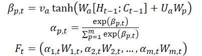
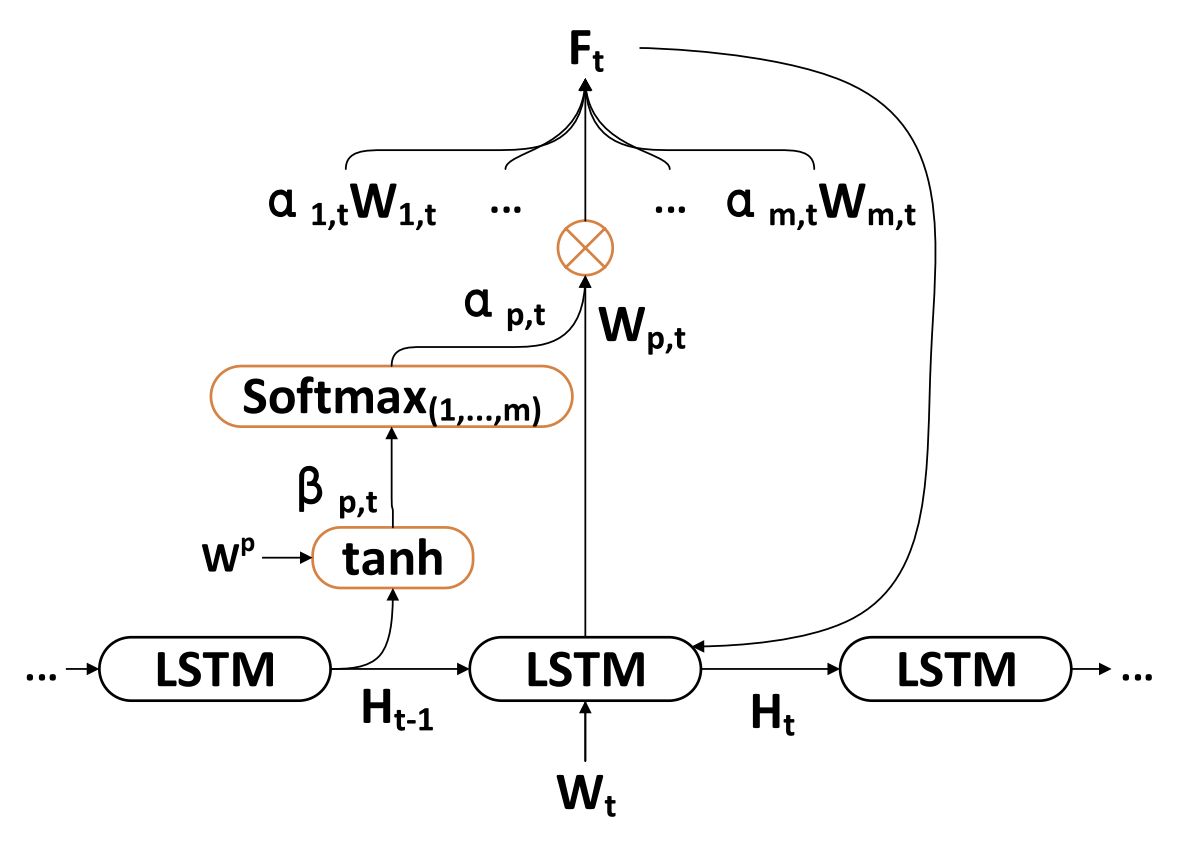
where va, Wa and Ua are parameters, and the SoftMax function is used to calculate importance αm,t of each feature dimension.
All dimensions Wt are updated to Ft and are fed into the Encoder. After that the hidden state of the time point t is updated.
Thus, at every time step t, we can choose relevant dimensions of spatial market features, iteratively update the original features and the hidden state of the Encoder, and generate the most relevant encoding vector for short-term features.
The decoder is and LSTMblock designed for predicting stock market trends. Long-term temporal features ZT-1 are extracted by the PLR method.
At every time step t, the decoder learns the relationship between the encoding vector Wt, a long-term feature Lt and a hidden state Ht:
![]()
where H't is the hidden state of the Decoder at the time step t, fde(•) is a nonlinear function, and ʘde denotes the decoder parameters.
The authors of TPM use LSTM as a nonlinear function fde to capture temporal dependencies and form a Long-Term Feature Decoder. The calculation procedure is similar to the Encoder stage.
The authors of TPM introduce an attention mechanism at the Decoder stage to obtain the associated hidden states of the Encoder of all time points.
The context vector fed to the Decoder is obtained through all the hidden states of the Encoder.
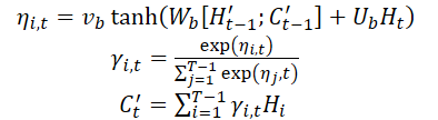
Once the context vector C't is obtained, it is combined with long-term temporary features Lt to generate a mixed feature yt:
![]()
Using the above formulas, at each time step t, the algorithm selects the most relevant hidden states of the Encoder of all time points and long-term temporal features to generate mixed feature vectors.
Next, the nonlinear mapping function F(•) between stock market trend and dual features is studied. Finally, a linear function is applied to generate the stock market trend prediction at time T.
The model was trained using the stochastic gradient descent method and a momentum optimizer. The training batch size was 64 and the learning rate was 0.001.
A quadratic error function with regularization terms is used as the loss function.
Author's visualization of the TPM method is presented below.
2. Implementing in MQL5
After examining the theoretical aspects of the proposed TPM method, we now move on to the practical implementation of our approach, where we present our interpretation of the proposed approaches. As usual, we preserve the general framework of the proposed methodology but introduce some deviations in the implementation details. Naturally, these adjustments may have varying impacts on the final performance of the model.
We will begin by constructing the Encoder.
2.1 TPM Encoder
We implement the Encoder for our model in the CNeuronTPMEncoder class which inherits the basic functionality from the previously created LSTM block CNeuronLSTMOCL. The choice of this parent class is intentional. As, you may recall, the Encoder in the TPM method is based on an LSTM block with an added attention mechanism.
Additionally, we decided to incorporate the feature extraction process for short-term features directly into the Encoder. The feature extraction will be performed using the previously developed data pyramidal structure builder CSCM. However, there is an important nuance: previously, the CSCM block was used to extract features from univariate time series. Now, we need to modify the data flow slightly to extract features from individual time points.
The overall structure of the Encoder is presented below.
class CNeuronTPMEncoder :  public CNeuronLSTMOCL
  {
protected:
   bool                 bTSinRow;
   //---
   CNeuronCSCMOCL       cFeatureExtraction;
   CNeuronBaseOCL       cMemAndHidden;
   CNeuronConcatenate   cConcatenated;
   CNeuronSoftMaxOCL    cSoftMax;
   CNeuronBaseOCL       cAttentionOut;
   CNeuronTransposeOCL  cTranspose;
   CBufferFloat         cTemp;
   //---
   virtual bool      feedForward(CNeuronBaseOCL *NeuronOCL) override;
   //---
   virtual bool      updateInputWeights(CNeuronBaseOCL *NeuronOCL) override;
   //---
   virtual bool      calcInputGradients(CNeuronBaseOCL *NeuronOCL) override;

public:
                     CNeuronTPMEncoder(void){};
                    ~CNeuronTPMEncoder(void){};
   virtual bool      Init(uint numOutputs, uint myIndex, COpenCLMy *open_cl,
                          uint variables, uint lenth, uint hidden_size, bool ts_in_row,
                          ENUM_OPTIMIZATION optimization_type, uint batch);
   //---
   virtual bool      Save(int const file_handle) override;
   virtual bool      Load(int const file_handle) override;
   //---
   virtual int       Type(void) override       const                      {  return defNeuronTPMEncoder; }
   virtual void      SetOpenCL(COpenCLMy *obj);
  };
Here, we see the familiar set of overridden methods and several nested objects, whose purpose we will become clear as we proceed with the implementation.
As before, all nested objects are declared as static. This approach allows us to leave both the constructor and destructor of the class "empty". The actual initialization of an instance of our new class is carried out within the Init method.
bool CNeuronTPMEncoder::Init(uint numOutputs, uint myIndex, COpenCLMy *open_cl,
                             uint variables, uint lenth, uint hidden_size, bool ts_in_row,
                             ENUM_OPTIMIZATION optimization_type, uint batch)
  {
   if(!CNeuronLSTMOCL::Init(numOutputs, myIndex, open_cl, hidden_size, optimization_type, batch))
      return false;
   if(!SetInputs(variables * lenth))
      return false;
In the parameters, this method receives the main parameters of the created object. In this case, there are 3 such parameters:
- variables — the number of univariate sequences within the analyzed multimodal time series.
- lenth — the size of the analyzed sequence (history depth).
- hidden_size — the size of the hidden space in the LSTM block.
In addition, we have added flag ts_in_row, which indicates the location of individual univariate sequences in the rows of the input data tensor.
In the method body, we call the identically named method from the parent class, which provides a required control block for verifying the parameters of the created layer and initialization of the inherited objects.
Here we also pass the size of the input tensor of the parent class, which is equal to the product of the size of the univariate sequence by the number of such sequences in the input data.
Please note that inside the LSTM block, we used fully connected layers, while the input data tensor is not relevant in this case.
The next step is to initialize the short-term feature extraction block.
   uint windows[] = {variables, 6, 5, 4};
   if(!cFeatureExtraction.Init(0, 0, OpenCL, windows, lenth, variables, ts_in_row, optimization, batch))
      return false;
To do this, we first set the window sizes of the convolutional feature extraction layers and call the CSCM block initialization method.
Please note that when calling the CSCM block initialization method, we rearranged the parameters of the size and number of univariate sequences. This is due to the need to extract features from individual time steps (bars), rather than univariatte sequences, as provided by the MSFformer method.
Next, we initialize the nested objects of the attention block. Here we first create a layer in whose buffers we concatenate the hidden state and context of the LSTM block in the previous step.
   if(!cMemAndHidden.Init(0, 1, OpenCL, hidden_size * 2, optimization, batch))
      return false;
To calculate the importance coefficients of individual features, we will use a concatenation layer, the results of which we normalize using the SoftMax function.
   if(!cConcatenated.Init(0, 2, OpenCL, variables * lenth, variables * lenth, hidden_size * 2, optimization, batch))
      return false;
   cConcatenated.SetActivationFunction(TANH);
   if(!cSoftMax.Init(0, 3, OpenCL, variables * lenth, optimization, batch))
      return false;
   cSoftMax.SetHeads(variables);
Note that at this stage the data normalization is performed within univariate sequences.
Next, we add a layer to record the attention outputs.
   if(!cAttentionOut.Init(0, 4, OpenCL, variables * lenth, optimization, batch))
      return false;
If necessary, we initialize the data transposition layer.
   bTSinRow = ts_in_row;
   if(!bTSinRow)
     {
      if(!cTranspose.Init(0, 5, OpenCL, variables, lenth, optimization, iBatch))
         return false;
     }
We also add an auxiliary buffer for recording intermediate values.
//---
   if(!cTemp.BufferInit(variables * lenth, 0) || !cTemp.BufferCreate(OpenCL))
      return false;
//---
   return true;
  }
After successful initialization of all nested objects, we pass the logical result of the performed operations to the caller and terminate the method.
After completing the initialization the object, we move on to constructing the feed-forward pass algorithm for the new class, which we implement in the feedForward method.
bool CNeuronTPMEncoder::feedForward(CNeuronBaseOCL *NeuronOCL)
  {
//--- FEATURE EXTRACTION
   if(!cFeatureExtraction.FeedForward(NeuronOCL))
      return false;
As usual, in the parameters of this method we receive a pointer to the object of the previous neural layer. However, in this case, we do not check the received pointer but pass it to the feed-forward method of the inner short-term feature extraction layer. The body of the called method itself implements control over the received pointer.
The next step is to combine the hidden state and context of our object that were preserved from the previous feed-forward pass.
//--- Memory and Hidden
   if(!Concat(m_iHiddenState, m_iMemory, m_iHiddenState, m_iMemory,
              cMemAndHidden.getOutputIndex(), 1, 1, 0, 0, Neurons()))
      return false;
This concludes our preparatory work. Now, let's move on to the attention block. In this block, we calculate the importance coefficients of individual features.
   if(!cConcatenated.FeedForward(cFeatureExtraction.AsObject(), cMemAndHidden.getOutput()))
      return false;
   if(!cSoftMax.FeedForward(cConcatenated.AsObject()))
      return false;
   int map = cSoftMax.getOutputIndex();
If necessary, we transpose the importance coefficient tensor.
   if(!bTSinRow)
     {
      if(!cTranspose.FeedForward(cSoftMax.AsObject()))
         return false;
      map = cTranspose.getOutputIndex();
     }
Then we need to perform element-by-element multiplication of the obtained coefficients by the corresponding short-term features. For element-wise multiplication of 2 tensors, we will use the feed-forward pass kernel of the Dropout layer.
We created this kernel to multiply the input data by the neuron exclusion mask. In this case, we use importance coefficients as a mask.
Let's define the dimension of the task space.
   uint global_work_offset[1] = {0};
   uint global_work_size[1];
   global_work_size[0] = int(cSoftMax.Neurons() + 3) / 4;
Pass the parameters to the kernel.
   ResetLastError();
   if(!OpenCL.SetArgumentBuffer(def_k_Dropout, def_k_dout_input, cFeatureExtraction.getOutputIndex()))
     {
      printf("Error of set parameter kernel %s: %d; line %d", __FUNCTION__, GetLastError(), __LINE__);
      return false;
     }
   if(!OpenCL.SetArgumentBuffer(def_k_Dropout, def_k_dout_map, map))
     {
      printf("Error of set parameter kernel %s: %d; line %d", __FUNCTION__, GetLastError(), __LINE__);
      return false;
     }
   if(!OpenCL.SetArgumentBuffer(def_k_Dropout, def_k_dout_out, cAttentionOut.getOutputIndex()))
     {
      printf("Error of set parameter kernel %s: %d; line %d", __FUNCTION__, GetLastError(), __LINE__);
      return false;
     }
   if(!OpenCL.SetArgument(def_k_Dropout, def_k_dout_dimension, cSoftMax.Neurons()))
     {
      printf("Error of set parameter kernel %s: %d; line %d", __FUNCTION__, GetLastError(), __LINE__);
      return false;
     }
After that we put it in the execution queue.
   if(!OpenCL.Execute(def_k_Dropout, 1, global_work_offset, global_work_size))
     {
      printf("Error of execution kernel %s: %d", __FUNCTION__, GetLastError());
      return false;
     }
After executing the kernel in the AttentionOut layer buffer, we obtain short-term features taking into account their importance coefficient. Now, we can use the basic functionality of the LSTM block for representing the feature tensor at the output of our Encoder.
//--- LSTM
   if(!CNeuronLSTMOCL::feedForward(cAttentionOut.AsObject()))
      return false;
//---
   return true;
  }
Do not forget to monitor the operations processes at every stage. After successful execution, we pass the logical result of the performed operations to the caller and complete the method.
After implementing the feed-forward pass, we usually move on to constructing the backpropagation methods. This class is no exception. In the next step, we implement error gradient propagation to all nested objects and the input data tensor in accordance with their influence on the final result of the model. We implement the specified functionality in the calcInputGradients method.
In the parameters of this method, similar to the one discussed above, we receive a pointer to the object of the previous neural layer.
bool CNeuronTPMEncoder::calcInputGradients(CNeuronBaseOCL *NeuronOCL)
  {
   if(!NeuronOCL)
      return false;
In the method body, we first check the relevance of the received pointer.
Then, using the inherited functionality, we propagate the error gradient through the LSTM block algorithm to the output level of our attention block.
   if(!CNeuronLSTMOCL::calcInputGradients(cAttentionOut.AsObject()))
      return false;
After that, we distribute the error gradient in 2 directions: feature importance coefficients and the features themselves. The algorithm for placing the kernel in a queue is similar to that discussed above.
//---
   uint global_work_offset[1] = {0};
   uint global_work_size[1];
   global_work_size[0] = cSoftMax.Neurons();
   ResetLastError();
   if(!OpenCL.SetArgumentBuffer(def_k_CGConv_HiddenGradient, def_k_cgc_matrix_f, cFeatureExtraction.getOutputIndex()))
     {
      printf("Error of set parameter kernel %s: %d; line %d", __FUNCTION__, GetLastError(), __LINE__);
      return false;
     }
   if(!OpenCL.SetArgumentBuffer(def_k_CGConv_HiddenGradient, def_k_cgc_matrix_fg, cTemp.GetIndex()))
     {
      printf("Error of set parameter kernel %s: %d; line %d", __FUNCTION__, GetLastError(), __LINE__);
      return false;
     }
   if(!OpenCL.SetArgumentBuffer(def_k_CGConv_HiddenGradient, def_k_cgc_matrix_s,
                                 (bTSinRow ? cSoftMax.getOutputIndex() : cTranspose.getOutputIndex())))
     {
      printf("Error of set parameter kernel %s: %d; line %d", __FUNCTION__, GetLastError(), __LINE__);
      return false;
     }
   if(!OpenCL.SetArgumentBuffer(def_k_CGConv_HiddenGradient, def_k_cgc_matrix_sg,
                             (bTSinRow ? cSoftMax.getGradientIndex() : cTranspose.getGradientIndex())))
     {
      printf("Error of set parameter kernel %s: %d; line %d", __FUNCTION__, GetLastError(), __LINE__);
      return false;
     }
   if(!OpenCL.SetArgumentBuffer(def_k_CGConv_HiddenGradient, def_k_cgc_matrix_g, cAttentionOut.getGradientIndex()))
     {
      printf("Error of set parameter kernel %s: %d; line %d", __FUNCTION__, GetLastError(), __LINE__);
      return false;
     }
   if(!OpenCL.SetArgument(def_k_CGConv_HiddenGradient, def_k_cgc_activationf, NeuronOCL.Activation()))
     {
      printf("Error of set parameter kernel %s: %d; line %d", __FUNCTION__, GetLastError(), __LINE__);
      return false;
     }
   if(!OpenCL.SetArgument(def_k_CGConv_HiddenGradient, def_k_cgc_activations, int(None)))
     {
      printf("Error of set parameter kernel %s: %d; line %d", __FUNCTION__, GetLastError(), __LINE__);
      return false;
     }
   if(!OpenCL.Execute(def_k_CGConv_HiddenGradient, 1, global_work_offset, global_work_size))
     {
      printf("Error of execution kernel %s: %d", __FUNCTION__, GetLastError());
      return false;
     }
Here, we should pay attention to two points. First, the error gradient propagation buffer for the attention coefficients depends on the need to use the importance coefficient transposition layer. Second, we use the short-term features themselves both when multiplying by the importance coefficients and when calculating these coefficients. Therefore, at this stage, we save the error gradient of short-term features in a temporary data buffer.
In the next step, we, if necessary, transpose the error gradient of the importance coefficients of individual features.
   if(bTSinRow)
     {
      if(!cSoftMax.calcHiddenGradients(cTranspose.AsObject()))
         return false;
     }
After that we propagate the error gradient through the attention block algorithm to the level of short-term features.
   if(!cConcatenated.calcHiddenGradients((CObject*)cSoftMax.AsObject(),(CBufferFloat *)NULL,(CBufferFloat *)NULL) ||
      !DeActivation(cConcatenated.getOutput(), cConcatenated.getGradient(), cConcatenated.getGradient(),
                                                                            cConcatenated.Activation()))
      return false;
   if(!cFeatureExtraction.calcHiddenGradients(cConcatenated.AsObject(), cMemAndHidden.getOutput(),
                                                                        cMemAndHidden.getGradient()))
      return false;
Then we sum up the error gradient at the level of short-term features from 2 information threads.
   if(!DeActivation(cFeatureExtraction.getOutput(), GetPointer(cTemp), GetPointer(cTemp), NeuronOCL.Activation()) ||
      !SumAndNormilize(cFeatureExtraction.getGradient(), GetPointer(cTemp), cFeatureExtraction.getGradient(), 1, false))
      return false;
At the end of the method, we propagate the error gradient down to the level of the previous layer and pass the logical result of the operations to the caller.
   if(!NeuronOCL.calcHiddenGradients(cFeatureExtraction.AsObject()))
      return false;
//---
   return true;
  }
After distributing the error gradient, we just need to optimize the model parameters towards minimizing the overall error. We implement this functionality in the updateInputWeights method by calling the identically named methods of the nested objects that contain the trainable parameters.
bool CNeuronTPMEncoder::updateInputWeights(CNeuronBaseOCL *NeuronOCL)
  {
   if(!CNeuronLSTMOCL::updateInputWeights(cAttentionOut.AsObject()))
      return false;
   if(!cFeatureExtraction.UpdateInputWeights(NeuronOCL))
      return false;
   if(!cConcatenated.UpdateInputWeights(cFeatureExtraction.AsObject(), cMemAndHidden.getOutput()))
      return false;
//---
   return true;
  }
This concludes the description of the algorithms for implementing the main functionality of our Encoder. The complete code for all methods of this class is available in the attachment, along with the full code for all programs used in preparing this article.
2.2 TPM Decoder
After implementing the TPM Encoder algorithms, we move on to the second stage - building the Decoder. During your review of the theoretical aspects of the TPM method, you likely noticed significant similarities between the Encoder and Decoder algorithms. However, even with minor differences we need to develop a new class.
Similar to the Encoder, the new Decoder class CNeuronTPMDecoder is derived from the LSTM block class. The structure of the new class is shown below.
class CNeuronTPM :  public CNeuronLSTMOCL
  {
protected:
   CNeuronTPMEncoder    cEncoder;
   CNeuronPLROCL        cFeatureExtraction;
   CNeuronBaseOCL       cMemAndHidden;
   CNeuronConcatenate   cConcatenated;
   CNeuronSoftMaxOCL    cSoftMax;
   CNeuronBaseOCL       cAttentionOut;
   CNeuronConcatenate   cAttAndFeature;
   CBufferFloat         cTemp;
   //---
   virtual bool      feedForward(CNeuronBaseOCL *NeuronOCL) override;
   //---
   virtual bool      updateInputWeights(CNeuronBaseOCL *NeuronOCL) override;
   //---
   virtual bool      calcInputGradients(CNeuronBaseOCL *NeuronOCL) override;

public:
                     CNeuronTPM(void){};
                    ~CNeuronTPM(void){};
   virtual bool      Init(uint numOutputs, uint myIndex, COpenCLMy *open_cl,

                          uint variables, uint lenth, uint hidden_size, bool ts_in_row,
                          ENUM_OPTIMIZATION optimization_type, uint batch);
   //---
   virtual bool      Save(int const file_handle) override;
   virtual bool      Load(int const file_handle) override;
   //---
   virtual int       Type(void) override       const                      {  return defNeuronTPM; }
   virtual void      SetOpenCL(COpenCLMy *obj);
  };
It is easy to see the similarity with the Encoder class discussed above. Only 2 nested objects have been added. You can also notice the change in the type of feature extraction layer: in the Decoder we use PLR to extract long-term features.
You may have noticed that the Encoder class includes a specification of ownership, which is absent in the Decoder. There is a reason for this distinction. The Encoder and Decoder operate on the same input data but extract features at different levels of abstraction. To avoid overcomplicating the model structure at the upper level, I decided to merge the Encoder and Decoder into a unified block. The previously developed Encoder class has been added as an internal layer within the new class, combining the TPM algorithm into a single entity. This decision is reflected in the name of the new class: CNeuronTPM.
The parameters of the initialization method of the new class are completely identical to the Encoder initialization method discussed above.
bool CNeuronTPM::Init(uint numOutputs, uint myIndex, COpenCLMy *open_cl,
                      uint variables, uint lenth, uint hidden_size, bool ts_in_row,
                      ENUM_OPTIMIZATION optimization_type, uint batch)
  {
   if(!CNeuronLSTMOCL::Init(numOutputs, myIndex, open_cl, hidden_size, optimization_type, batch))
      return false;
   if(!SetInputs(hidden_size))
      return false;
In the body of the method, we also call the initialization method of the parent class. However, the size of its input data tensor already corresponds to the size of the hidden state of the Encoder. This is because the Decoder is fed with the weighted vector of features received from the Encoder.
We also initialize the Encoder object
   if(!cEncoder.Init(0, 0, OpenCL, variables, lenth, hidden_size, ts_in_row, optimization, iBatch))
      return false;
and the feature extraction layer.
   if(!cFeatureExtraction.Init(0, 1, OpenCL, variables, lenth, !ts_in_row, optimization, iBatch))
      return false;
The further algorithm for initializing the attention block objects resembles similar operations during the initialization of the Encoder, but there are differences in the sizes of the input data tensors.
   if(!cMemAndHidden.Init(0, 2, OpenCL, hidden_size * 2, optimization, iBatch))
      return false;
   if(!cConcatenated.Init(0, 3, OpenCL, hidden_size, hidden_size, hidden_size * 2, optimization, iBatch))
      return false;
   cConcatenated.SetActivationFunction(TANH);
   if(!cSoftMax.Init(0, 4, OpenCL, hidden_size, optimization, iBatch))
      return false;
   cSoftMax.SetHeads(1);
   if(!cAttentionOut.Init(0, 5, OpenCL, hidden_size, optimization, iBatch))
      return false;
As mentioned earlier, the LSTM block uses fully connected layers. Therefore, the tensor of short-term features obtained from the Encoder can be considered "anonymous" in the context of univariate sequences of the analyzed input multimodal time series. This allows us to normalize the importance coefficients across the entire tensor. At this stage, the orientation of the input tensor is not important to us.
Let's add a projection layer of weighted short-term and long-term features of the analyzed time series, which we will feed into the LSTM block.
   if(!cAttAndFeature.Init(0, 6, OpenCL, hidden_size, hidden_size, variables * lenth, optimization, iBatch))
      return false;
At the end of the class initialization operations, we add a buffer to store temporary data.
   if(!cTemp.BufferInit(variables * lenth, 0) || !cTemp.BufferCreate(OpenCL))
      return false;
//---
   return true;
  }
We return the logical result of initializing the nested objects to the caller.
After initializing the nested objects, we move on to implementing the feed-forward algorithm in the feedForward method. Similar to other identically named methods, in the parameters we receive a pointer to the object of the previous neural layer.
bool CNeuronTPM::feedForward(CNeuronBaseOCL *NeuronOCL)
  {
//--- Encoder
   if(!cEncoder.FeedForward(NeuronOCL))
      return false;
Then we pass the received pointer to the feed-forward method of our Encoder.
Next, we pass the same pointer to extract long-term features of the analyzed time series.
//--- FEATURE EXTRACTION
   if(!cFeatureExtraction.FeedForward(NeuronOCL))
      return false;
The operation of the attention block is similar to the Encoder block discussed above.
//--- Memory and Hidden
   if(!Concat(m_iHiddenState, m_iMemory, m_iHiddenState, m_iMemory,
              cMemAndHidden.getOutputIndex(), 1, 1, 0, 0, Neurons()))
      return false;
//--- Attention
   if(!cConcatenated.FeedForward(cEncoder.AsObject(), cMemAndHidden.getOutput()))
      return false;
   if(!cSoftMax.FeedForward(cConcatenated.AsObject()))
      return false;
We multiply the importance coefficients by the vector of short-term features of the Encoder.
   uint global_work_offset[1] = {0};
   uint global_work_size[1];
   global_work_size[0] = int(cSoftMax.Neurons() + 3) / 4;
   ResetLastError();
   if(!OpenCL.SetArgumentBuffer(def_k_Dropout, def_k_dout_input, cEncoder.getOutputIndex()))
     {
      printf("Error of set parameter kernel %s: %d; line %d", __FUNCTION__, GetLastError(), __LINE__);
      return false;
     }
   if(!OpenCL.SetArgumentBuffer(def_k_Dropout, def_k_dout_map, cSoftMax.getOutputIndex()))
     {
      printf("Error of set parameter kernel %s: %d; line %d", __FUNCTION__, GetLastError(), __LINE__);
      return false;
     }
   if(!OpenCL.SetArgumentBuffer(def_k_Dropout, def_k_dout_out, cAttentionOut.getOutputIndex()))
     {
      printf("Error of set parameter kernel %s: %d; line %d", __FUNCTION__, GetLastError(), __LINE__);
      return false;
     }
   if(!OpenCL.SetArgument(def_k_Dropout, def_k_dout_dimension, cSoftMax.Neurons()))
     {
      printf("Error of set parameter kernel %s: %d; line %d", __FUNCTION__, GetLastError(), __LINE__);
      return false;
     }
   if(!OpenCL.Execute(def_k_Dropout, 1, global_work_offset, global_work_size))
     {
      printf("Error of execution kernel %s: %d", __FUNCTION__, GetLastError());
      return false;
     }
We combine the weighted vector of short-term features with the long-term features in a concatenation layer.
//--- Attention and Features
   if(!cAttAndFeature.FeedForward(cAttentionOut.AsObject(), cFeatureExtraction.getOutput()))
      return false;
We then feed this prepared data into LSTM block.
//--- LSTM
   if(!CNeuronLSTMOCL::feedForward(cAttAndFeature.AsObject()))
      return false;
//---
   return true;
  }
We verify the logical result of the operations and return it to the calling program.
Next, we would typically move on to constructing the backpropagation methods. However, I believe you have noticed the similarities between the forward-pass methods of the Encoder and Decoder. Of course, there are some nuances. Similar nuances also exist in the backpropagation methods. Nevertheless, the algorithms are quite similar overall. So, I encourage you to explore them on your own in the provided attachment.
2.3 Architecture of Trainable Models
We have examined the implementation of the TPM method using MQL5. This method was developed to predict stock price trends. Naturally, we will integrate it into our environmental state Encoder, the architecture of which is described in the CreateEncoderDescriptions method.
In the parameters, the method receives a pointer to a dynamic array in which we will save the embedded model architecture.
bool CreateEncoderDescriptions(CArrayObj *encoder)
  {
//---
   CLayerDescription *descr;
//---
   if(!encoder)
     {
      encoder = new CArrayObj();
      if(!encoder)
         return false;
     }
In the method body, we check the relevance of the received pointer and, if necessary, create a new instance of the dynamic array object.
As usual, we feed the model with raw data describing the state of the environment. To record the initial data, we use a basic fully connected layer, the size of which should be sufficient to write the analyzed tensor.
//--- Encoder
   encoder.Clear();
//--- Input layer
   if(!(descr = new CLayerDescription()))
      return false;
   descr.type = defNeuronBaseOCL;
   int prev_count = descr.count = (HistoryBars * BarDescr);
   descr.activation = None;
   descr.optimization = ADAM;
   if(!encoder.Add(descr))
     {
      delete descr;
      return false;
     }
The obtained initial data is preprocessed in the batch normalization layer.
//--- layer 1
   if(!(descr = new CLayerDescription()))
      return false;
   descr.type = defNeuronBatchNormOCL;
   descr.count = prev_count;
   descr.batch = 1e4;
   descr.activation = None;
   descr.optimization = ADAM;
   if(!encoder.Add(descr))
     {
      delete descr;
      return false;
     }
Te preprocessed data is then passed to our TPM module.
//--- layer 2
   if(!(descr = new CLayerDescription()))
      return false;
   descr.type = defNeuronTPM;
   descr.count = LatentCount;
   descr.window = BarDescr;
   descr.window_out = HistoryBars;
   descr.step = int(false);
   descr.activation = None;
   descr.optimization = ADAM;
   if(!encoder.Add(descr))
     {
      delete descr;
      return false;
     }
Data obtained from the TPM module is propagated through a 3-layer MLP, at the output of which we expect to obtain the predicted values for the analyzed time series.
//--- layer 3
   if(!(descr = new CLayerDescription()))
      return false;
   descr.type = defNeuronBaseOCL;
   descr.count = LatentCount;
   descr.activation = LReLU;
   descr.optimization = ADAM;
   if(!encoder.Add(descr))
     {
      delete descr;
      return false;
     }
//--- layer 4
   if(!(descr = new CLayerDescription()))
      return false;
   descr.type = defNeuronBaseOCL;
   descr.count = LatentCount;
   descr.optimization = ADAM;
   descr.activation = SIGMOID;
   if(!encoder.Add(descr))
     {
      delete descr;
      return false;
     }
//--- layer 5
   if(!(descr = new CLayerDescription()))
      return false;
   descr.type = defNeuronBaseOCL;
   descr.count = BarDescr * NForecast;
   descr.optimization = ADAM;
   descr.activation = TANH;
   if(!encoder.Add(descr))
     {
      delete descr;
      return false;
     }
To the forecast values, we add statistical variables of the original time series that were previously removed in the batch normalization layer.
//--- layer 6
   if(!(descr = new CLayerDescription()))
      return false;
   descr.type = defNeuronRevInDenormOCL;
   descr.count = BarDescr * NForecast;
   descr.activation = None;
   descr.optimization = ADAM;
   descr.layers = 1;
   if(!encoder.Add(descr))
     {
      delete descr;
      return false;
     }
Then we align the obtained predicted output in frequency representation.
//--- layer 7
   if(!(descr = new CLayerDescription()))
      return false;
   descr.type = defNeuronFreDFOCL;
   descr.window = BarDescr;
   descr.count =  NForecast;
   descr.step = int(true);
   descr.probability = 0.7f;
   descr.activation = None;
   descr.optimization = ADAM;
   if(!encoder.Add(descr))
     {
      delete descr;
      return false;
     }
//---
   return true;
  }
The Actor and Critic models have been copied from previous works without changes. You can find them in the attachment.
2.4 Model training EAs
When training models, we should pay attention to the specifics of training recurrent models. As you know, the main feature of recurrent models is their sensitivity to the sequence of input data. Therefore, in the model training process, we need to use data from the training dataset following the historical sequence. On the other hand, this approach reduces the training efficiency of most models, as it promotes overfitting within small time intervals with the inability to generalize to the entire training period.
To minimize the negative impact of the mentioned factors, during the training process we will randomly extract small subsets from the experience replay buffer in accordance with the historical sequence. Then we will sample a new training package. Let's consider the implementation of the proposed approach using the Environment State Encoder training method as an example. The Expert Advisor file "...\Experts\TPM\StudyEncoder.mq5" is also attached below.
void Train(void)
  {
//---
   vector<float> probability = GetProbTrajectories(Buffer, 0.9);
In the body of the method, we first generate a vector of probabilities for choosing passes from the training set, ranked by the profitability of the passes. After that we declare the necessary local variables.
   vector<float> result, target, state;
   bool Stop = false;
Next, we add a variable indicating the size of one subset training batch.
int Batch = 100;
Then we create a system of nested loops. In the outer loop, we sample a trajectory from the training set and the start state of the training subset on the sampled trajectory.
   uint ticks = GetTickCount();
//---
   for(int iter = 0; (iter < Iterations && !IsStopped() && !Stop); iter += Batch)
     {
      int tr = SampleTrajectory(probability);
      int st = (int)((MathRand() * MathRand() / MathPow(32767, 2)) * (Buffer[tr].Total - 2 - NForecast));
      if(st <= 0)
        {
         iter -= Batch;
         continue;
        }
We clear the hidden state and context buffers of the LSTM block.
Encoder.Clear();
After that, we run a nested loop to sequentially iterate over the states in their historical sequence from the selected state of the environment.
      for(int i = st; (i < MathMin(st + Batch, Buffer[tr].Total - NForecast) && !IsStopped() && !Stop); i++)
        {
         state.Assign(Buffer[tr].States[i].state);
         if(MathAbs(state).Sum() == 0)
           {
            iter += i - st - Batch;
            break;
           }
         bState.AssignArray(state);
In the body of the nested loop, we transfer the analyzed state of the environment to the data buffer. Based on the data obtained, we predict the next price movement trajectory.
         //--- State Encoder
         if(!Encoder.feedForward((CBufferFloat*)GetPointer(bState), 1, false, (CBufferFloat*)NULL))
           {
            PrintFormat("%s -> %d", __FUNCTION__, __LINE__);
            Stop = true;
            break;
           }
We then load the target values of the next trajectory from the experience replay buffer.
         //--- Collect target data
         if(!Result.AssignArray(Buffer[tr].States[i + NForecast].state))
            continue;
         if(!Result.Resize(BarDescr * NForecast))
            continue;
Next, we check the accuracy of our forecasts. During the backpropagation pass, we adjust the model parameters towards minimizing the error in predicting the next movement.
         if(!Encoder.backProp(Result, (CBufferFloat*)NULL))
           {
            PrintFormat("%s -> %d", __FUNCTION__, __LINE__);
            Stop = true;
            break;
           }
Inform the user about the progress of the learning process and move on to the next iteration of the loop system.
         if(GetTickCount() - ticks > 500)
           {
            double percent = double(iter + i - st) * 100.0 / (Iterations);
            string str = StringFormat("%-14s %6.2f%% -> Error %15.8f\n", "Encoder",
                                            percent, Encoder.getRecentAverageError());
            Comment(str);
            ticks = GetTickCount();
           }
        }
     }
After all iterations of the loop system have been successfully completed, we clear the comments field on the symbol chart. We output the training results to the terminal log and initialize the Expert Advisor shutdown.
   Comment("");
//---
   PrintFormat("%s -> %d -> %-15s %10.7f", __FUNCTION__, __LINE__, "Encoder", Encoder.getRecentAverageError());
   ExpertRemove();
//---
  }
Similar edits have been made to the Actor and Critic training EA. Although recurrent blocks were not added to these models, making these edits was necessary to ensure the correct operation of the Environmental State Encoder. This is because both the Actor and the Critic use it as input data.
You can find the full code of the model training EA in the attachment. The attachment also contains the complete code of all programs, classes and methods used in this article.
3. Testing
In this article, we explored a method for predicting upcoming stock trajectories using TPM and implemented our interpretation of the proposed approaches. It is now time to test the results of our work using real data. As usual, we train the presented models on historical EURUSD H1 timeframe data for the year 2023.
We begin by training the Environment Encoder model, which analyzes historical price movement data without assessing the Actor's actions. This approach allows us to fully train the model on the initial dataset without requiring frequent updates. The training process was relatively fast and showed good results. Below is a chart comparing the predicted and actual price movement trajectories.
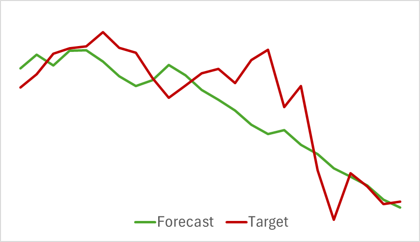
The chart demonstrates a close overlap of the two lines, with the predicted trajectory appearing smoother. This smoothing effect has the potential to enhance the stability of Actor training.
As you know, our primary objective is to optimize the Actor's policy. After training the Environment Encoder, we move to the second stage of the training process - Actor policy training. This process is iterative in nature. Since the Actor's actions are shifted and can move beyond the bounds of the previously collected training data, we need to periodically update the experience replay buffer by populating it with states and rewards closer to the Actor's current policy actions.
After several alternating iterations of training the Actor and Critic models, along with updates to the training dataset, we developed a policy capable of generating profits on the historical training data.
To evaluate the model's performance outside the training dataset, we test it using historical data from January 2024 while keeping other conditions the same.
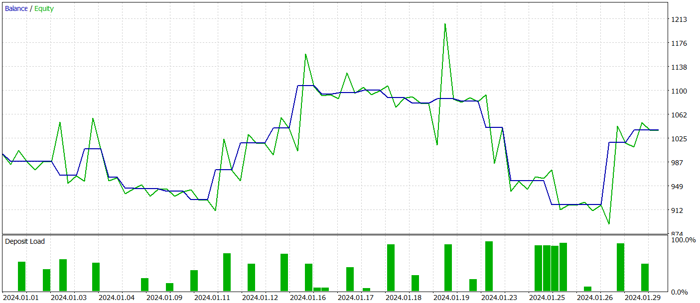
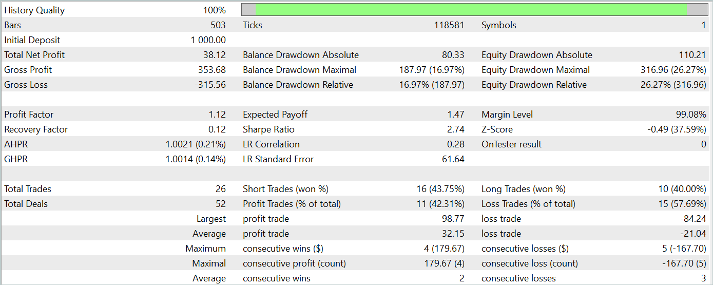
During the testing period, the model executed 26 trades, of which only 11 were profitable, i.e. just over 42%. However, both the maximum and average profit per trade exceeded the corresponding loss metrics, resulting in an overall profit for the test period. The profit factor for the test period was 1.12.
Nevertheless, the balance chart reveals a significant drawdown during the early part of the third decade of the month. This raises concerns. Despite generating a profit, the model still requires further refinement.
Conclusion
In this article, we explored an intriguing method for predicting price movement trends using TPM. This method effectively combines the strengths of convolutional models for analyzing short-term dependencies and PLR for identifying long-term trends.
In the practical section of the article, we implemented our interpretation of the proposed approaches using MQL5, trained the models, and conducted testing. The results show that the trained model was able to generate profits on data outside the training dataset. However, the balance chart did not display the desired consistent upward trend and had drawdowns.
Overall, while the proposed method demonstrates potential, the model we developed requires further refinement.
References
Programs used in the article
| # | Name | Type | Description |
|---|---|---|---|
| 1 | Research.mq5 | EA | Example collection EA |
| 2 | ResearchRealORL.mq5 | EA | EA for collecting examples using the Real-ORL method |
| 3 | Study.mq5 | EA | Model training EA |
| 4 | StudyEncoder.mq5 | EA | Encoder training EA |
| 5 | Test.mq5 | EA | Model testing EA |
| 6 | Trajectory.mqh | Class library | System state description structure |
| 7 | NeuroNet.mqh | Class library | A library of classes for creating a neural network |
| 8 | NeuroNet.cl | Code Base | OpenCL program code library |
Translated from Russian by MetaQuotes Ltd.
Original article: https://www.mql5.com/ru/articles/15255
Warning: All rights to these materials are reserved by MetaQuotes Ltd. Copying or reprinting of these materials in whole or in part is prohibited.
This article was written by a user of the site and reflects their personal views. MetaQuotes Ltd is not responsible for the accuracy of the information presented, nor for any consequences resulting from the use of the solutions, strategies or recommendations described.

 Mastering Log Records (Part 3): Exploring Handlers to Save Logs
- Free trading apps
- Over 8,000 signals for copying
- Economic news for exploring financial markets
You agree to website policy and terms of use