Data Science and ML (Part 42): Forex Time series Forecasting using ARIMA in Python, Everything you need to Know

Contents
- What is time series forecasting?
- Introduction to ARIMA models
- Key components of an ARIMA model
- ARIMA model in Python
- Building ARIMA model on EURUSD
- Out-of-sample predictions using ARIMA
- Residual plots from the ARIMA model
- SARIMA model
- Conclusion
What is Time Series Forecasting?
Time series forecasting is the process of using past data to predict future values in a sequence of data points. This sequence is typically ordered by time, hence the name time series.
Core Variables in Time series data
While we can have as many feature variables as we want in our data, any data for time series analysis or forecasting must have these two variables.
- Time
This is an independent variable, representing the specific points in time when the data points were observed. - Target Variable
This is the value you're trying to predict based on past observations and potentially other factors. (e.g., Daily closing stock price, hourly temperature, website traffic per minute).
The goal of time series forecasting is to leverage historical patterns and trends within the data to make informed predictions about future values.
We have discussed before about time series forecasting using regular AI models. In this article, we are going to discuss time series forecasting using a model designed for time series problems known as ARIMA.
Time series forecasting can be divided into two types.
- Univariate time series forecasting
This is a time series forecasting problem where one predictor is used to predict its future values. For example, using the current closing prices of a stock to predict future closing prices.
This is the type of forecasting that ARIMA models are capable of. - Multivariate time series forecasting
This is a time series forecasting problem where multiple predictors are used to predict a target variable in the future.
Similarly to what we did in this article.
Introduction to ARIMA Models
ARIMA stands for Autoregressive Integrated Moving Average
It belongs to a class of models that explain a given time series based on its past values, i.e. its lags and the lagged forecast errors.
The equation can be used to forecast future values. Any "non-seasonal" time series that exhibits patterns and is not a random white noise can be modeled with ARIMA models.
So, ARIMA, short for AutoRegressive Integrated Moving Average, is a forecasting algorithm based on the idea that the information in the past values of the time series alone can be used to predict the future values.
ARIMA Models are specified by three order parameters: (p, d, q),
Where:
- p is the order of the AR term
- q is the order of the MA term
- d is the number of differencing required to make the time series stationary
The meaning of p,d, and q in ARIMA model
The meaning of p
p is the order of the Auto Regressive (AR) term. It refers to the number of lags of Y to be used as predictors.
The meaning of d
The term Auto Regressive in ARIMA means it is a linear regression model that uses its lags as predictors. Linear regression models, as we know, work best when the predictors are not correlated and are independent of each other so, we need to make the time series stationary.
The most common approach to make the series stationary is to differentiate it. That is, subtract the previous value from the current value. Sometimes, depending on the complexity of the series, more than one differencing may be needed.
The value of d, therefore, is the minimum number of differencing needed to make the series stationary. If the time series is already stationary, then d = 0.
The meaning of q
q is the order of the Moving Average (MA) term. It refers to the number of lagged forecast errors that should go into the ARIMA Model.
Key Components of an ARIMA Model
To understand ARIMA, we need to deconstruct its building blocks. Once we have the components broken down it becomes easier to understand how this time series forecasting method works as a whole.
The name ARIMA can be broken into three parts (AR, I, MA) as described below.
Autoregressive AR(p) part
The Autoregressive (AR) component builds a trend from past values in the AR framework for predictive models. For clarification, the "autoregression framework" works like a regression model where you use the lags of the time series' own past values as the regressors.
This part is calculated by the following formula:
![]()
Where:
-
 is the current value of the time series at time t.
 -
 is the constant term.
 -
 to
to  are the autoregressive parameters (coefficients) that indicate how much each lagged value contributes to the current value
 -
 to
to  are the past values of the time series lags
 -
 is the error term at time t.
Integrated I(d) part
The Integrated (I) part involves the differencing of the time series component while keeping in mind that our time series should be stationary, which means that the mean and variance should remain constant over a period of time.
Basically, we subtract one observation from another so that trends and seasonality are eliminated. By performing differencing, we get stationarity. This step is necessary because it helps the model fit the data and not the noise.
Moving average MA(q) part
The moving average (MA) component focuses on the relationship between an observation and a residual error. Looking at how the present observation is related to those of the past errors, we can then infer some helpful information about any possible trend in our data.
We can consider the residuals among one of these errors, and the moving average model concept estimates or considers their impact on our latest observation. This is particularly useful for tracking and trapping short-term changes in the data or random shocks. In the (MA) part of a time series, we can gain valuable information about its behavior which in turn allows us to forecast and predict with greater accuracy.
![]()
Where:
-
 is a constant.
 -
 is the MA parameter.
 -
 is the previous error.
 -
 is the current error.
ARIMA Model in Python
So, an ARIMA model is simply a combination of the three parts described above, AR, I, and MA parts as described above. Its equation now becomes.
![]()
Now, the challenge in ARIMA models is finding the right parameters (the p,d, and q values). Since these values the the ones that run the model, let us understand how to find these values.
Finding the order of the AR term (p)
We can find the required number of AR terms by inspecting the Partial Autocorrelation (PACF) plot.
Partial autocorrelation can be described as the correlation between the series and its lag(s) after excluding the contributions from the intermediate lags. So, PACF sort of conveys the pure correlation between a lag and the series. This way, we will know if that lag is needed in the AR term or not.
Start by installing all dependencies in the command prompt (CMD). The file requirements.txt is attached at the end of this post.
pip install -r requirements.txt
Imports.
# Importing required libraries
import pandas as pd
import numpy as np
import MetaTrader5 as mt5

# Use auto_arima to automatically select best ARIMA parameters

import seaborn as sns
import matplotlib.pyplot as plt
import warnings
import os

# Suppress warning messages for cleaner output
warnings.filterwarnings("ignore")

# Set seaborn plot style for better visualization
sns.set_style("darkgrid")
Getting the data from MetaTrader5.
# Getting (EUR/USD OHLC data) from MetaTrader5

mt5_exe_file = r"c:\Users\Omega Joctan\AppData\Roaming\Pepperstone MetaTrader 5\terminal64.exe" # Change this to your MetaTrader5 path
if not mt5.initialize(mt5_exe_file):
    print("Failed to initialize Metatrader5, error = ",mt5.last_error)
    exit()

# select a symbol into the market watch
symbol = "EURUSD"
timeframe = mt5.TIMEFRAME_D1

if not mt5.symbol_select(symbol, True):
    print(f"Failed to select {symbol}, error = {mt5.last_error}")
    mt5.shutdown()
    exit()

rates = mt5.copy_rates_from_pos(symbol, timeframe, 1, 1000) # Get 1000 bars historically
df = pd.DataFrame(rates)

print(df.head(5))
print(df.shape)
PACF plot.
from statsmodels.graphics.tsaplots import plot_pacf
import matplotlib.pyplot as plt

plt.figure(figsize=(6,4))
plot_pacf(series.diff().dropna(), lags=5)

plt.title("Partial Autocorrelation Plot")
plt.xlabel('Lag')  # X-axis label
plt.ylabel('PACF')  # Y-axis label

plt.savefig("pacf plot.png")
plt.show()
Outputs.
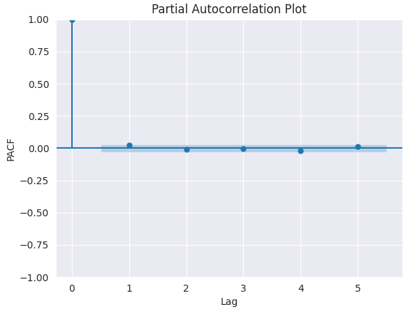
To determine the right value of p, we look for the lag after which PACF cuts off on the plot (drops near zero and stays insignificant). That lag value is the correct candidate for p.
From the chart above, the right p value is 0 (all the lags beyond 0 are insignificant).
Finding the order of differencing (d) in an ARIMA model
As explained earlier, the purpose of differencing a time series is to make it stationary since the ARIMA model assumes stationarity, but, we should be careful not to under- and over-difference a time series.
The right order of differencing is the minimum differencing required to get a near-stationarity series which roams around a defined mean and the Auto Correlation Function (ACF) plot reaches to zero fairly quick.
If the autocorrelations are positive for many number of lags (10 or more), then the series needs further differencing. On the other hand, if the lag 1 of autocorrelation is too negative, then the series is probably over-differenced.
If we can't decide between two orders of differencing, then we choose the order that gives the least standard deviation in the differenced series.
Using the closing prices of EURUSD, let's find the right order of differencing.
Firstly, we have to check if the given series is stationary (closing prices in this case) using the Augmented Dickey Fuller Test (ADF Test), from the statsmodels package in Python. We check for stationarity because we only want to find the order of differencing only to a non-stationary series.
The null hypothesis (Ho) of the ADF test is that the time series is non-stationary. So, if the p-value of the test is less than the significance level (0.05) then we reject the null hypothesis and infer that the timeseries is indeed stationary.
So, in our case, if the P value > 0.05, we go ahead with finding the right order of differencing.
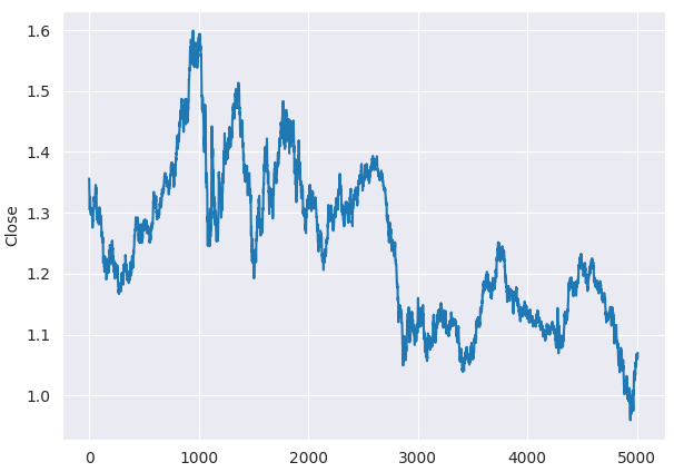
Even before the ADF test, we can tell that the closing prices of EURUSD aren't stationary by looking at the line plot.
plt.figure(figsize=(7,5))
sns.lineplot(df, x=df.index, y="Close")
plt.savefig("close prices.png")
Outputs.
Checking stationarity.
from statsmodels.tsa.stattools import adfuller

series = df["Close"]
result = adfuller(series)

print(f'p-value: {result[1]}')
Outputs.
p-value: 0.3707268514544181
As you can see, the p-value is way greater than the significance level (0.05). Let us differentiate the series once, then twice, and see how the autocorrelation plot looks like.
# Original Series
fig, axes = plt.subplots(3, 2, sharex=True, figsize=(9, 9))

axes[0, 0].plot(series); axes[0, 0].set_title('Original Series')
plot_acf(series, ax=axes[0, 1])

# 1st Differencing
axes[1, 0].plot(series.diff().dropna()); axes[1, 0].set_title('1st Order Differencing')
plot_acf(series.diff().dropna(), ax=axes[1, 1])

# 2nd Differencing
axes[2, 0].plot(series.diff().diff()); axes[2, 0].set_title('2nd Order Differencing')
plot_acf(series.diff().diff().dropna(), ax=axes[2, 1])

plt.savefig("acf plots.png")
plt.show()
Outputs.
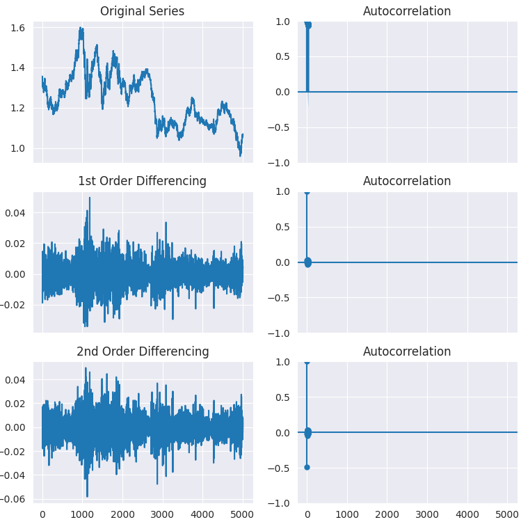
As it can be seen from the plots, the first order of differencing does the job as there is no significant difference in stationarity outcome observed on the second order of differencing. This can be verified once again by the ADF test.
result = adfuller(series.diff().dropna())
print(f'p-value d=1: {result[1]}')

result = adfuller(series.diff().diff().dropna())
print(f'p-value d=2: {result[1]}')
Outputs.
p-value d=1: 0.0
p-value d=2: 0.0
Finding the order of the MA term (q)
Just like how we looked at the PACF plot for the number of AR terms (d), we will look at the ACF plot for the number of MA terms. Again, the MA term is technically, the error of the lagged forecast.
The ACF plot tells us how many MA terms are required to remove any autocorrelation in the stationarized series.
plt.figure(figsize=(7,5))
plot_pacf(series.diff().dropna(), lags=20)

plt.title("Partial Autocorrelation Plot")
plt.xlabel('Lag')  # X-axis label
plt.ylabel('PACF')  # Y-axis label

plt.savefig("pacf plot finding q.png")
plt.show()
Outputs.
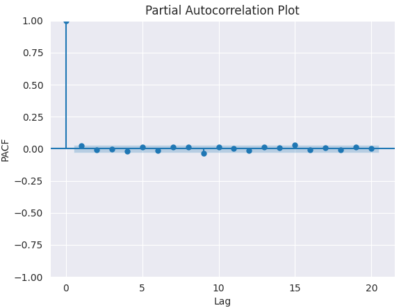
The best value of q is 0.
Now the methods discussed above on finding p, d, and q values are crude and manual, we can automate this process and find the parameters without much hassle using a utility function from pmdarima named auto_arima.
from pmdarima.arima import auto_arima

model = auto_arima(series, seasonal=False, trace=True)
print(model.summary())
Outputs.
Performing stepwise search to minimize aic
 ARIMA(2,1,2)(0,0,0)[0] intercept   : AIC=-35532.282, Time=3.21 sec
 ARIMA(0,1,0)(0,0,0)[0] intercept   : AIC=-35537.068, Time=0.49 sec
 ARIMA(1,1,0)(0,0,0)[0] intercept   : AIC=-35537.492, Time=0.59 sec
 ARIMA(0,1,1)(0,0,0)[0] intercept   : AIC=-35537.511, Time=0.74 sec
 ARIMA(0,1,0)(0,0,0)[0]             : AIC=-35538.731, Time=0.25 sec
 ARIMA(1,1,1)(0,0,0)[0] intercept   : AIC=-35535.683, Time=1.22 sec

Best model:  ARIMA(0,1,0)(0,0,0)[0]
Total fit time: 6.521 seconds
Just like that, we got the same parameters as the ones we got doing manual analysis.
Building an ARIMA model on EURUSD
Now that we have determined the values of p,d, and q, we have everything needed to fit (train) the ARIMA model.
from statsmodels.tsa.arima.model import ARIMA

arima_model = ARIMA(series, order=(0,1,0))
arima_model = arima_model.fit()
print(arima_model.summary())
Outputs.
                               SARIMAX Results
==============================================================================
Dep. Variable:                  Close   No. Observations:                 4007
Model:                 ARIMA(0, 1, 0)   Log Likelihood               13987.647
Date:                Mon, 26 May 2025   AIC                         -27973.293
Time:                        16:59:38   BIC                         -27966.998
Sample:                             0   HQIC                        -27971.062
                               - 4007
Covariance Type:                  opg
==============================================================================
                 coef    std err          z      P>|z|      [0.025      0.975]
------------------------------------------------------------------------------
sigma2      5.427e-05   7.78e-07     69.768      0.000    5.27e-05    5.58e-05
===================================================================================
Ljung-Box (L1) (Q):                   1.47   Jarque-Bera (JB):              1370.86
Prob(Q):                              0.22   Prob(JB):                         0.00
Heteroskedasticity (H):               0.49   Skew:                             0.09
Prob(H) (two-sided):                  0.00   Kurtosis:                         5.86
===================================================================================

Warnings:
[1] Covariance matrix calculated using the outer product of gradients (complex-step).
Now let's train this model on some data and use it to make predictions on out-of-sample data, similarly to how we do with classical machine learning models.
Starting with splitting the data into training and testing samples.
series = df["Close"]

train_size = int(len(series) * 0.8)
train, test = series[:train_size], series[train_size:]
Fitting the model to the training data.
from statsmodels.tsa.arima.model import ARIMA

arima_model = ARIMA(train, order=(0,1,0))
arima_model = arima_model.fit()
print(arima_model.summary())
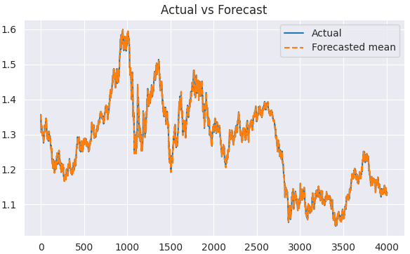
Making predictions on the training data.
predicted = arima_model.predict(start=1, end=len(train))
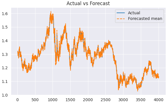
Visualizing the outcome.
plt.figure(figsize=(7,4))
plt.plot(train.index, train, label='Actual')
plt.plot(train.index, predicted, label='Forecasted mean', linestyle='--')
plt.title('Actual vs Forecast')
plt.legend()
plt.show()
Outputs.
Now that we have actual and their forecasted values, we can evaluate the model using any evaluation technique or loss function of our choice.
But, before that, let us find a way to use this ARIMA model to make predictions on the out-of-sample data.
Out-of-sample Predictions Using ARIMA
Unlike classic machine learning algorithms, these traditional time series forecasting models take on a different approach when it comes to making predictions on the information it hasn't seen before.
In classic machine learning frameworks and Python libraries, a method named predict, when called with an array of data, it makes a prediction/guesses the next (future) value(s), but, predict function offered by the ARIMA module does a quite different job.
In ARIMA models, this method doesn't necessarily predict the future; it is handy only when it comes to making predictions based on the in-sample data (the information already present in the model), in other words, the training data.
To grasp this, let's discuss the difference between predicting and forecasting.
Predicting is estimating unknown values (future or otherwise) using any model, while forecasting refers to predicting future values in a time series data by leveraging temporal patterns and dependencies.
Prediction can be applied to problems like classifying market direction or estimating the next closing prices, while forecasting is used to predict the next stock prices based on the current value(s).
In the ARIMA model, the predict method is typically used in making forecasting for the past values that the model has learned from, that is why it takes the starting index and end index. It can also take the number of steps in the past you want to predict (evaluate).
predicted = arima_model.predict(start=1, end=len(train))
print(arima_model.predict(steps=10))
To forecast the future value(s), we have to use a method named forecast().
As said earlier, traditional time series-based models such as ARIMA depend on the previous value(s) to forecast the next value(s), as it can be seen from its formula in figure 03.
This means that we have to constantly update the model with new information for it to stay relevant. For example, to get an ARIMA model to make a forecast on tomorrow's closing price of EURUSD this model must be fed with today's closing price of the same instrument (symbol), the same applies for tomorrow and the following day.
This is quite different from what we do in classical machine learning.
Now let's make predictions on out-of-sample data.
# Fit initial model

model = ARIMA(train, order=(0, 1, 0))
results = model.fit()

# Initialize forecasts
forecasts = [results.forecast(steps=1).iloc[0]]  # First forecast

# Update with test data iteratively
for i in range(len(test)):
    # Append new observation without refitting
    results = results.append(test.iloc[i:i+1], refit=False)

    # Forecast next step
    forecasts.append(results.forecast(steps=1).iloc[0])

forecasts = forecasts[:-1] # remove the last element which is the predicted next value

# Compare forecasts vs actual test data
plt.plot(test.index, test, label="Actual")
plt.plot(test.index, forecasts, label="Forecast", linestyle="--")
plt.legend()
The append method inserts new (current information) into the model. In this case, the current closing price of EURUSD is used to forecast the next closing price.
refit=False, ensures the model is not trained once again. Making this an effective way to update the ARIMA model.
Let's make a function with a couple of evaluation metrics that we can use to assess the performance of the ARIMA model.
import sklearn.metrics as metric
from statsmodels.tsa.stattools import acf
from scipy.stats import pearsonr

def forecast_accuracy(forecast, actual):
    # Convert to numpy arrays if they aren't already
    forecast = np.asarray(forecast)
    actual = np.asarray(actual)

    metrics = {
        'mape': metric.mean_absolute_percentage_error(actual, forecast),
        'me': np.mean(forecast - actual),  # Mean Error
        'mae': metric.mean_absolute_error(actual, forecast),
        'mpe': np.mean((forecast - actual) / actual),  # Mean Percentage Error
        'rmse': metric.mean_squared_error(actual, forecast, squared=False),
        'corr': pearsonr(forecast, actual)[0],  # Pearson correlation
        'minmax': 1 - np.mean(np.minimum(forecast, actual) / np.maximum(forecast, actual)),
        'acf1': acf(forecast - actual, nlags=1)[1],  # ACF of residuals at lag 1
        "r2_score": metric.r2_score(forecast, actual)
    }

    return metrics
forecast_accuracy(forecasts, test)
Outputs.
{'mape': 0.0034114761554881936,
'me': 6.360279441117738e-05,
'mae': 0.0037872155688622737,
'mpe': 6.825424905960248e-05,
'rmse': 0.005018824533752777,
'corr': 0.99656297100796,
'minmax': 0.0034008221524469695,
'acf1': 0.04637470541528736,
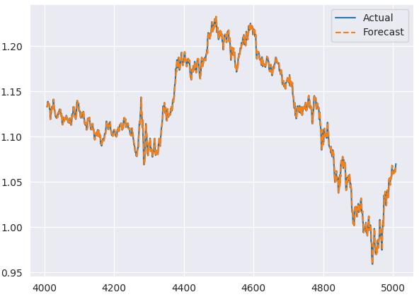
'r2_score': 0.9931220697334551} The mape value of 0.003 indicates the model is approximately 99.996% accurate, approximately the same value can be seen in the r2_score.
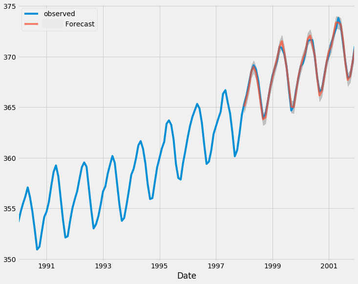
Below is the plot comparing actual and predicted outcomes from the testing sample.
Residual Plots from the ARIMA Model
ARIMA comes with methods for visualizing the residuals for a better understanding of the model.
results.plot_diagnostics(figsize=(8,8))
plt.show()
Outputs.
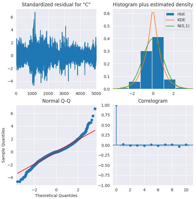
Standardized residual
The residual errors seem to fluctuate around a mean of zero and have a uniform variance.
Histogram
The density plot suggests normal distribution with mean slightly shifted towards the right.
Theoretical Quantiles
Most of the dots fall perfectly in line with the red line. Any significant deviations would imply the distribution is skewed.
Correlogram
The Correlogram (or ACF plot) shows that the residual errors are not autocorrelated. The ACF plot would imply that there is some pattern in the residual errors which are not explained in the model, so, we will need to look for more X’s (predictors) to the model.
Overall, the model seems to be a good fit.
SARIMA model
The plain ARIMA model has a problem. It does not support seasonality.
Seasonality refers to recurring patterns in financial data that repeat at fixed intervals, such as hourly, daily, weekly, monthly, quarterly, and yearly.
We often see instruments exhibit certain repetitive patterns. For example, retail stocks often surge in Q4 (holiday shopping season), while some energy stocks may follow seasonal weather patterns, in forex instruments we can spot increased market volatility during certain trading sessions etc.
If the time series data has observable or defined seasonality, then we should go for Seasonal ARIMA model (in short SARIMA) since it uses seasonal differencing.
SARIMAX(p, d, q)x(P, D, Q, S) model components
- Autoregression (AR)
As described before, autoregression examines past values of the time series to predict current values. - Moving average (MA)
The moving average continues to model past errors in predictions. - Integration (I)
Integration is always present to make the time series stationary. - Seasonal component (S)
The seasonal component captures variations that recur at regular intervals.
Seasonal differencing is similar to regular differencing, but, instead of subtracting consecutive terms, we subtract the value from the previous season.
Before calling the SARIMAX model, let's determine the right parameters for it using auto_arima.
from pmdarima.arima import auto_arima

# Auto-fit SARIMA (automatically detects P, D, Q, S)

auto_model = auto_arima(
    series,
    seasonal=True,          # Enable seasonality
    m=5,                    # Weeky cycle (5 days) for daily data
    trace=True,             # Show search progress
    stepwise=True,          # Faster optimization
    suppress_warnings=True,
    error_action="ignore"
)

print(auto_model.summary())
Outputs.
Performing stepwise search to minimize aic
 ARIMA(2,1,2)(1,0,1)[5] intercept   : AIC=-35529.092, Time=3.81 sec
 ARIMA(0,1,0)(0,0,0)[5] intercept   : AIC=-35537.068, Time=0.29 sec
 ARIMA(1,1,0)(1,0,0)[5] intercept   : AIC=-35536.573, Time=0.97 sec
 ARIMA(0,1,1)(0,0,1)[5] intercept   : AIC=-35536.570, Time=4.38 sec
 ARIMA(0,1,0)(0,0,0)[5]             : AIC=-35538.731, Time=0.21 sec
 ARIMA(0,1,0)(1,0,0)[5] intercept   : AIC=-35536.048, Time=0.67 sec
 ARIMA(0,1,0)(0,0,1)[5] intercept   : AIC=-35536.024, Time=0.87 sec
 ARIMA(0,1,0)(1,0,1)[5] intercept   : AIC=-35534.248, Time=0.92 sec
 ARIMA(1,1,0)(0,0,0)[5] intercept   : AIC=-35537.492, Time=0.37 sec
 ARIMA(0,1,1)(0,0,0)[5] intercept   : AIC=-35537.511, Time=0.55 sec
 ARIMA(1,1,1)(0,0,0)[5] intercept   : AIC=-35535.683, Time=0.57 sec

Best model:  ARIMA(0,1,0)(0,0,0)[5]
Total fit time: 13.656 seconds
                               SARIMAX Results
==============================================================================
Dep. Variable:                      y   No. Observations:                 5009
Model:               SARIMAX(0, 1, 0)   Log Likelihood               17770.365
Date:                Tue, 27 May 2025   AIC                         -35538.731
Time:                        11:16:40   BIC                         -35532.212
Sample:                             0   HQIC                        -35536.446
                               - 5009
Covariance Type:                  opg
==============================================================================
                 coef    std err          z      P>|z|      [0.025      0.975]
------------------------------------------------------------------------------
sigma2      4.846e-05   6.06e-07     80.005      0.000    4.73e-05    4.96e-05
===================================================================================
Ljung-Box (L1) (Q):                   2.42   Jarque-Bera (JB):              2028.68
Prob(Q):                              0.12   Prob(JB):                         0.00
Heteroskedasticity (H):               0.34   Skew:                             0.08
Prob(H) (two-sided):                  0.00   Kurtosis:                         6.11
===================================================================================

Warnings:
[1] Covariance matrix calculated using the outer product of gradients (complex-step).
Despite no need to re-fit the model manually once more because auto_arima returns a SARIMAX, re-fitting a SARIMAX model manually gives us more control to the results, so let's do it once again.
from statsmodels.tsa.statespace.sarimax import SARIMAX

model = SARIMAX(
    train,
    order=auto_model.order,                  # Non-seasonal (p,d,q)
    seasonal_order=auto_model.order+(5,),      # Seasonal (P,D,Q,S)
    enforce_stationarity=False
)

results = model.fit()
print(results.summary())
Outputs.
                                     SARIMAX Results
=========================================================================================
Dep. Variable:                             Close   No. Observations:                 4007
Model:             SARIMAX(0, 1, 0)x(0, 1, 0, 5)   Log Likelihood               12613.829
Date:                           Tue, 27 May 2025   AIC                         -25225.658
Time:                                   11:16:41   BIC                         -25219.364
Sample:                                        0   HQIC                        -25223.427
                                          - 4007
Covariance Type:                             opg
==============================================================================
                 coef    std err          z      P>|z|      [0.025      0.975]
------------------------------------------------------------------------------
sigma2         0.0001   1.68e-06     63.423      0.000       0.000       0.000
===================================================================================
Ljung-Box (L1) (Q):                   3.42   Jarque-Bera (JB):               676.61
Prob(Q):                              0.06   Prob(JB):                         0.00
Heteroskedasticity (H):               0.48   Skew:                            -0.01
Prob(H) (two-sided):                  0.00   Kurtosis:                         5.01
===================================================================================

Warnings:
[1] Covariance matrix calculated using the outer product of gradients (complex-step).
Since the order returned from auto_model is for ARIMA(p,d,q), despite setting seasonal value to true. We have to append the value of 5 to a tuple when declaring the SARIMAX model to ensure the model is now (p,d,q,s).
Before visualizing and analyzing actual and predicted outcomes, we have to drop the first items equal to the seasonal window in our array. Values before this value are incomplete.
predicted = results.predict(start=1, end=len(train))

clean_train = train[5:]
clean_predicted = predicted[5:]

plt.figure(figsize=(7,4))
plt.plot(clean_train.index[5:], clean_train[5:], label='Actual')
plt.plot(clean_train.index[5:], clean_predicted[5:], label='Forecasted mean', linestyle='--')
plt.title('Actual vs Forecast')
plt.legend()
plt.savefig("sarimax train actual&forecast plot.png")
plt.show()
Outputs.
We can evaluate this model similarly to how we evaluated the ARIMA model.
# Initialize forecasts
forecasts = [results.forecast(steps=1).iloc[0]]  # First forecast

# Update with test data iteratively
for i in range(len(test)):
    # Append new observation without refitting
    results = results.append(test.iloc[i:i+1], refit=False)

    # Forecast next step
    forecasts.append(results.forecast(steps=1).iloc[0])

clean_test = test[5:]
forecasts = forecasts[5:-1] # remove the last element which is the predicted next value and the first 5 items
forecast_accuracy(forecasts, clean_test)
Outputs.
{'mape': 0.004900183060803821,
 'me': -6.94082142749275e-06,
 'mae': 0.005432456867698095,
 'mpe': -7.226495372320155e-06,
 'rmse': 0.007127465498996785,
 'corr': 0.9931778828074744,
 'minmax': 0.004880027322298863,
 'acf1': 0.10724254539104018,
 'r2_score': 0.9864021833085908}
A 98.6% accuracy according to the r2_score. A decent value.
Finally, we can use the ARIMA model to make real-time predictions according to data received from MetaTrader5.
Firstly, we have to import the schedule library to help us to make predictions after one day since we trained this model on a daily timeframe.
import schedule # Make realtime predictions based on the recent data from MetaTrader5 def predict_close(): rates = mt5.copy_rates_from_pos(symbol, timeframe, 0, 1) if not rates: print(f"Failed to get recent OHLC values, error = {mt5.last_error}") time.sleep(60) rates_df = pd.DataFrame(rates) global results # Get the variable globally, outside the function global forecasts # Append new observation to the model without refitting new_obs_value = rates_df["close"].iloc[-1] new_obs_index = results.data.endog.shape[0] # continue integer index new_obs = pd.Series([new_obs_value], index=[new_obs_index]) # Its very important to continue making predictions where we ended on the training data results = results.append(new_obs, refit=False) # Forecast next step forecasts.append(results.forecast(steps=1).iloc[0]) print(f"Current Close Price: {new_obs_value} Forecasted next day Close Price: {forecasts[-1]}")
Scheduling making predictions.
schedule.every(1).days.do(predict_close) # call the predict function after a given time

while True:

    schedule.run_pending()
    time.sleep(60)

mt5.shutdown()
Outputs.
Current Close Price: 1.1374900000000001 Forecasted next day Close Price: 1.1337899981049262
Current Close Price: 1.1372200000000001 Forecasted next day Close Price: 1.1447100065656721
Given these predicted close prices, you can extend this to a trading strategy and pull off trading operations using MetaTrader5-Python.
Final Thoughts
Both ARIMA and SARIMA are decent traditional time series models that have been used in multiple fields and industries; However, you must understand their limitations and drawbacks, including:
- They assume stationarity (after differencing)
We don't always work with stationary data and we often want to use the data as it is, differencing the data can distort the natural structure and trends we anticipate. - Linearity assumption
ARIMA is inherently a linear model; It assumes that future values depend linearly on past lags and errors. This is wrong in financial and forex markets patterns, as complex patterns can be observed more often than not, this means this models could fall flat somewhere. - Univariate models
Both these models take one feature at a time. We both know that financial markets are complicated and we need multiple features and perspectives to look at the markets. These models only look at the market from one standpoint (one-dimensional) causing us to miss out on other features which could be helpful.
While you can add exogenous feature(s) to the SARIMAX model, it is often insufficient.
Despite their limitations, when used with the right parameters, problem type, and information. A simple ARIMA model can outperform complex models such as RNNs for time series forecasting.
Best regards.
Sources & References
- https://www.geeksforgeeks.org/python-arima-model-for-time-series-forecasting/
- https://www.machinelearningplus.com/time-series/arima-model-time-series-forecasting-python/
- https://datascientest.com/en/sarimax-model-what-is-it-how-can-it-be-applied-to-time-series
- https://www.kaggle.com/code/prashant111/arima-model-for-time-series-forecasting
Attachments Table
| Filename | Description & Usage |
|---|---|
| forex_ts_forecasting_using_arima.py | Python script containing all discussed examples in Python language. |
| requirements.txt | A text file containing Python dependencies and their version number |
Warning: All rights to these materials are reserved by MetaQuotes Ltd. Copying or reprinting of these materials in whole or in part is prohibited.
This article was written by a user of the site and reflects their personal views. MetaQuotes Ltd is not responsible for the accuracy of the information presented, nor for any consequences resulting from the use of the solutions, strategies or recommendations described.

- Free trading apps
- Over 8,000 signals for copying
- Economic news for exploring financial markets
You agree to website policy and terms of use
Amazing content.
Exactly what I was looking for.
Probably not going to use it in trading, but very interesting.
First heard about ARIMA in Perry J Kaufman's book Trading Systems & Methods .
Anyone had any success trading with ARIMA ?