
Neural Networks in Trading: Spatio-Temporal Neural Network (STNN)

Introduction
Time series forecasting plays an important role in various fields, including finance. We are already accustomed to the fact that many real-world systems allow us to measure multidimensional data that contain rich information about the dynamics of the target variable. However, effective analysis and forecasting of multivariate time series are often hindered by the "curse of dimensionality". This makes the selection of the historical data window for analysis a critical factor. Quite often, when using an insufficient window of analyzed data, the forecasting model demonstrates unsatisfactory performance and fails.
To address the complexities of multivariate data, the Spatio-Temporal Information (STI) Transformation equation was developed based on the delay embedding theorem. The STI equation transforms the spatial information of multivariate variables into the temporal dynamics of the target variable. This effectively increases the sample size and mitigates the challenges posed by short-term data.
Transformer-based models, already familiar in handling data sequences, use the Self-Attention mechanism to analyze relationships between variables while disregarding their relative distances. These attention mechanisms capture global information and focus on the most relevant features, alleviating the curse of dimensionality.
In the study "Spatiotemporal Transformer Neural Network for Time-Series Forecasting", a Spatiotemporal Transformer Neural Network (STNN) was proposed to enable efficient multi-step forecasting of multivariate short-term time series. This approach leverages the advantages of the STI equation and the Transformer framework.
The authors highlight several key benefits of their proposed methods:
- STNN uses the STI equation to convert the spatial information of multivariate variables into the temporal evolution of the target variable, effectively increasing the sample size.
- A continuous attention mechanism is proposed to improve the accuracy of numerical prediction.
- The spatial Self-Attention structure in the STNN collects efficient spatial information from multivariate variables, while the temporal Self-Attention structure collect information about the temporal evolution. The Transformer structure combines spatial and temporal information.
- The STNN model can reconstruct the phase space of a dynamical system for time series forecasting.
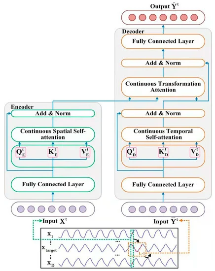
1. STNN Algorithm
The purpose of the STNN model is to effectively solve the nonlinear transformation equation STI through Transformer training.
![]()
The STNN model exploits the transformation equation STI and includes 2 dedicated attention modules to perform multi-step-ahead prediction. As you can see from the equation above, the D-dimensional input data at time t (Xt) is fed into the Encoder, which extracts effective spatial information from the input variables.
After this, the effective spatial information is transferred to the Decoder, which introduces a time series of length L-1 from the target variable Y (𝐘t). The Decoder extracts information about the temporal evolution of the target variable. It then predicts future values of the target variable by combining the spatial information of the input variables (𝐗t) and the temporal information of the target variable (𝐘t).
Note that the target variable is one of the variables in the multivariate input data X.
Nonlinear transformation of STI is solved by the Encoder-Decoder pair. The Encoder consists of 2 layers. The first is a fully connected layer, and the second one is a continuous spatial Self-Attention layer. The authors of the STNN method use a continuous spatial Self-Attention layer to extract effective spatial information from multivariate input data 𝐗t.
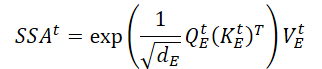
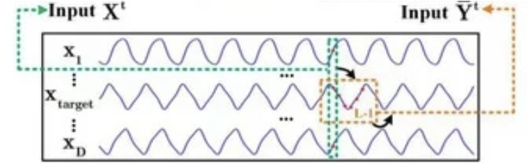
A fully connected layer is used to smooth the input multivariate time series data 𝐗t and to filter put noise. A single-layer neural network is shown in the following figure.
![]()
Where WFFN is the matrix of coefficients
bFFN is the bias
ELU is the activation function.
The continuous spatial Self-Attention layer accepts 𝐗t,FFN as input data. Because the Self-Attention layer accepts a multivariate time series, the Encoder can extract spatial information from the input data. To obtain effective spatial information (SSAt), a mechanism of continuous attention of the spatial Self-Attention layer is proposed. Its operation can be described as follows.
First, it generates 3 matrices of trainable parameters (WQE, WKE and WVE), which are used in the continuous spatial Self-Attention layer.
Then, by multiplying the input data 𝐗t,FFN by the the above mentioned weight matrices, it generates the Query, Key and Value entities of the continuous spatial Self-Attention layer.
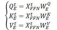
By performing the matrix scalar product, we obtain an expression for the key spatial information (SSAt) for the input data 𝐗t.
Where dE is the dimension of Query, Key and Value matrices.
The authors of the STNNmethod emphasize that, unlike the classical mechanism of discrete probabilistic attention, the proposed mechanism of continuous attention can guarantee uninterrupted transmission of Encoder data.
At the Encoder output, we sum the key spatial information tensor with the smoothed input data, followed by data normalization, which prevents the rapid gradient vanishing and accelerates the model convergence rate.
![]()
The Decoder combines effective spatial information and temporal evolutionary target variable. Its architecture includes 2 fully connected layers, a continuous temporal Self-Attention layer and a layer of transformation attention.
We feed the Decoder with the input data of the historical sequence of the target variable. As in the case of the Encoder, efficient representation of the input data (𝐘t,FFN) is obtained after filtering out noise with a fully connected layer.
The received data is then sent to the continuous temporal Self-Attention layer, which focuses on historical information about the temporal evolution between different time steps of the target variable. Since the influence of time is irreversible, we determine the current state of the time series using historical information, but not future information. Thus, the continuous temporal attention layer uses the masked attention mechanism to filter out future information. Let's take a closer look at this operation.
First, we generate 3 matrices of trainable parameters (WQD, WKD and WVD), for the spatio-temporal Self-Attention layer. Then we will calculate the corresponding Query, Key and Value entity matrices.
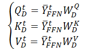
We perform a matrix scalar product to obtain information about the temporal evolution of the target variable over the analyzed period of history.
Unlike the Encoder, here we add a mask that removes the influence of subsequent elements of the analyzed data. In this way, we do not allow the model to "look into the future" when constructing the temporal evolution function of the target variable.
Next, we use residual connection and normalize the information about the temporal evolution of the target variable.
![]()
The continuous transformation attention layer for predicting future values of the target variable integrates spatial dependency information (SSAt) with data on the temporal evolution of the target variable (TSAt).

Residual relationships and data normalization are also used here.
![]()
At the output of the Decoder, the authors of the method use a second fully connected layer to predict the values of the target variable
![]()
When training the STNN model, the authors of the method used MSE as a loss function and L2 regularization of parameters.
The author's visualization of the method is presented below.
2. Implementing in MQL5
After considering the theoretical aspects of the STNN method, we move on to the practical part of our article in which we implement the proposed approaches in MQL5.
This article will present our own vision of the implementation, which may differ from the author's implementation of the method. Moreover, within the framework of this implementation, we tried to make maximum use of our existing developments, which also affected the result. We will talk about this while implementing the proposed approaches.
As you may have noticed from the theoretical description of the STNN algorithm presented above, it includes 2 main blocks: Encoder and Decoder. We will also divide our work into the implementation of 2 corresponding classes. Let's start with the implementation of the Encoder.
2.1 STNN Encoder
We will implement the Encoder algorithm within the CNeuronSTNNEncoder class. The authors of the method made some adjustments to the Self-Attention algorithm. However, it remains quite recognizable and includes the basic components of the classical approach. Therefore, to implement a new class, we will use existing developments and inherit the main functionality of the basic Self-Attention algorithm from the CNeuronMLMHAttentionMLKV class. The general structure of the new class is presented below.
class CNeuronSTNNEncoder  :  public CNeuronMLMHAttentionMLKV
  {
protected:
   virtual bool      feedForward(CNeuronBaseOCL *NeuronOCL) override;
   virtual bool      AttentionOut(CBufferFloat *q, CBufferFloat *kv, CBufferFloat *scores, CBufferFloat *out) override;
   //---
   virtual bool      calcInputGradients(CNeuronBaseOCL *prevLayer) override;
   virtual bool      updateInputWeights(CNeuronBaseOCL *NeuronOCL) override;

public:
                     CNeuronSTNNEncoder(void)  {};
                    ~CNeuronSTNNEncoder(void)  {};
   //---
   virtual int       Type(void)   override const   {  return defNeuronSTNNEncoder;   }
  };
As you can see, there are no declarations of new variables and objects within the new class. Moreover, the presented structure does not even contain an override of the object initialization methods. There are reasons for this. As mentioned above, we make maximum use of our existing developments.
First, let's look at the differences between the proposed approaches and those we have implemented previously. First of all, the authors of the STNN method placed a fully connected layer before the Self-Attention block. Technically, there is no problem with object declaration as it only affects the implementation of the feed-forward and backward pass algorithms. This means that the implementation of this moment does not affect the initialization method algorithm .
The second point is that the authors of the STNN method provided only one fully connected layer. However, in the classical approach, a block of 2 fully connected layers is created. My personal opinion is that using a block of 2 fully connected layers certainly increases the computational costs, but does not reduce the quality of the model. As an experiment, to maximize the preservation of existing developments, we can use 2 layers instead of 1.
In addition, the authors of the method have removed the SoftMax function from attention coefficient normalization step. Instead, they use a simple Query and Key matrix product exponent. In my opinion, the difference of SoftMax is only in data normalization and more complex calculations. So, in my implementation, I will use the previously implemented approach with SoftMax.
Next, we move on to the implementation of feed-forward algorithms. I noticed here that the authors of the method implemented masking of subsequent elements only in the Decoder. We remember that the target variable may be included in the set of Encoder's initial data. I thought there was some illogicality. But everything becomes clear after a close study of the author's visualization of the method.
Encoder's inputs are located at some distance from the analyzed state. I cannot judge the reasons why the authors of the method chose this implementation. But my personal opinion is that using the full information available at the time of data analysis will give us more information and potentially improve the quality of our forecasts. So in my implementation, I shift the Encoder's inputs to the current moment and add a mask of the initial data, which will allow us to analyze dependencies only with previous data.
To implement data masking, we need to make changes to the OpenCL program. Here we will make only minor changes to the MH2AttentionOut kernel. We will not use an additional masking buffer. We will do it in a simpler way. Let's add just 1 constant that will determine whether we need to use a mask. Masking will be organized directly in the kernel algorithm.
__kernel void MH2AttentionOut(__global float *q,
                              __global float *kv,
                              __global float *score,
                              __global float *out,
                              int dimension,
                              int heads_kv,
                              int mask ///< 1 - calc only previous units, 0 - calc all
                             )
  {
//--- init
   const int q_id = get_global_id(0);
   const int k = get_global_id(1);
   const int h = get_global_id(2);
   const int qunits = get_global_size(0);
   const int kunits = get_global_size(1);
   const int heads = get_global_size(2);
   const int h_kv = h % heads_kv;
   const int shift_q = dimension * (q_id * heads + h);
   const int shift_k = dimension * (2 *  heads_kv * k + h_kv);
   const int shift_v = dimension * (2 *  heads_kv * k + heads_kv + h_kv);
   const int shift_s = kunits * (q_id *  heads + h) + k;
   const uint ls = min((uint)get_local_size(1), (uint)LOCAL_ARRAY_SIZE);
   float koef = sqrt((float)dimension);
   if(koef < 1)
      koef = 1;
   __local float temp[LOCAL_ARRAY_SIZE];
In the kernel body, we will make only minor adjustments when calculating the sum of exponents.
//--- sum of exp
   uint count = 0;
   if(k < ls)
     {
      temp[k] = 0;
      do
        {
         if(mask == 0 || q_id <= (count * ls + k))
            if((count * ls) < (kunits - k))
              {
               float sum = 0;
               int sh_k = 2 * dimension * heads_kv * count * ls;
               for(int d = 0; d < dimension; d++)
                  sum = q[shift_q + d] * kv[shift_k + d + sh_k];
               sum = exp(sum / koef);
               if(isnan(sum))
                  sum = 0;
               temp[k] = temp[k] + sum;
              }
         count++;
        }
      while((count * ls + k) < kunits);
     }
   barrier(CLK_LOCAL_MEM_FENCE);
   count = min(ls, (uint)kunits);
Here we will add conditions and will calculate exponents only for the preceding elements. Please note that when creating inputs for the model, we form them from time series of historical price data and indicators. In time series, the current bar has index "0". Therefore, to mask elements in the historical chronology, we reset the dependence coefficients of all elements whose index is less than the analyzed Query. We see this when calculating the sum of the exponents and the dependence coefficients (underlined in the code).
//---
   do
     {
      count = (count + 1) / 2;
      if(k < ls)
         temp[k] += (k < count && (k + count) < kunits ? temp[k + count] : 0);
      if(k + count < ls)
         temp[k + count] = 0;
      barrier(CLK_LOCAL_MEM_FENCE);
     }
   while(count > 1);
//--- score
   float sum = temp[0];
   float sc = 0;
   if(mask == 0 || q_id >= (count * ls + k))
      if(sum != 0)
        {
         for(int d = 0; d < dimension; d++)
            sc = q[shift_q + d] * kv[shift_k + d];
         sc = exp(sc / koef) / sum;
         if(isnan(sc))
            sc = 0;
        }
   score[shift_s] = sc;
   barrier(CLK_LOCAL_MEM_FENCE);
The rest of the kernel code remains unchanged.
//--- out
   for(int d = 0; d < dimension; d++)
     {
      uint count = 0;
      if(k < ls)
         do
           {
            if((count * ls) < (kunits - k))
              {
               float sum =
                  kv[shift_v + d] * (count == 0 ? sc : score[shift_s + count * ls]);
               if(isnan(sum))
                  sum = 0;
               temp[k] = (count > 0 ? temp[k] : 0) + sum;
              }
            count++;
           }
         while((count * ls + k) < kunits);
      barrier(CLK_LOCAL_MEM_FENCE);
      //---
      count = min(ls, (uint)kunits);
      do
        {
         count = (count + 1) / 2;
         if(k < ls)
            temp[k] += (k < count && (k + count) < kunits ? temp[k + count] : 0);
         if(k + count < ls)
            temp[k + count] = 0;
         barrier(CLK_LOCAL_MEM_FENCE);
        }
      while(count > 1);
      //---
      out[shift_q + d] = temp[0];
     }
  }
Note that with this implementation, we simply zeroed out the dependency coefficients of next elements. This allowed us to implement masking with minimal edits to the feed-forward pass kernel. Moreover, this approach does not require any adjustment of the backpropagation kernels. Since "0" in the dependence coefficient will simply zero out the error gradient on such elements of the sequence.
This completes adjustments on the OpenCL program side. Now, we can move to working with the main program.
Here we first add the call of the above kernel in the CNeuronSTNNEncoder::AttentionOut method. The algorithm of the method for placing the kernel in the execution queue has not changed. You can study its code yourself in the attachment. I would just like to draw attention to the indication of "1" in the def_k_mh2ao_mask parameter to perform data masking.
Next, we move on to implementing the feed-forward pass method of our new class. We have to override the method to move the FeedForward block before Self-Attention. It should also be noted that, unlike the classical Transformer, the FeedForward block has no residual relationships and data normalization.
Before implementing the algorithm, it is important to recall that, in order to avoid unnecessary data copying during the initialization of the parent class, we replaced the result and error gradient buffer pointers of our layer with analogous buffers from the last layer of the FeedForward block. This approach takes advantage of the fact that the result buffer sizes of the attention block and the FeedForward block are identical. Therefore, we can simply adjust the indexing when accessing the respective data buffers.
Now, let's view our implementation. As before, the method parameters include a pointer to the object of the preceding layer, which provides the input data.
bool CNeuronSTNNEncoder::feedForward(CNeuronBaseOCL *NeuronOCL)
  {
   if(CheckPointer(NeuronOCL) == POINTER_INVALID)
      return false;
Right at the beginning of the method, we verify the validity of the received pointer. Once this is done, we proceed directly to constructing the feed-forward algorithm. Here, it is important to highlight another distinction in our implementation. The authors of the STNN method do not specify either the number of Encoder layers or the number of attention heads. Based on the visualization and method description provided earlier, we could expect the presence of only a single attention head in a single Encoder layer. However, in our implementation, we adhere to the classical approach, utilizing multi-head attention within a multi-layered architecture. We then organize a loop to iterate through the nested Encoder layers.
Within the loop, as previously mentioned, the input data first passes through the FeedForward block, where data smoothing and filtering are performed.
   CBufferFloat *kv = NULL;
   for(uint i = 0; (i < iLayers && !IsStopped()); i++)
     {
      //--- Feed Forward
      CBufferFloat *inputs = (i == 0 ? NeuronOCL.getOutput() : FF_Tensors.At(6 * i - 4));
      CBufferFloat *temp = FF_Tensors.At(i * 6 + 1);
      if(IsStopped() ||
         !ConvolutionForward(FF_Weights.At(i * (optimization == SGD ? 6 : 9) + 1), inputs, temp,
                                                                      iWindow, 4 * iWindow, LReLU))
         return false;
      inputs = FF_Tensors.At(i * 6);
      if(IsStopped() ||
         !ConvolutionForward(FF_Weights.At(i * (optimization == SGD ? 6 : 9) + 2), temp, inputs,
                                                                       4 * iWindow, iWindow, None))
         return false;
After that we define the matrices of the Query, Key and Value entities.
      //--- Calculate Queries, Keys, Values
      CBufferFloat *q = QKV_Tensors.At(i * 2);
      if(IsStopped() ||
        !ConvolutionForward(QKV_Weights.At(i * (optimization == SGD ? 2 : 3)), inputs, q,
                                                          iWindow, iWindowKey * iHeads, None))
         return false;
      if((i % iLayersToOneKV) == 0)
        {
         uint i_kv = i / iLayersToOneKV;
         kv = KV_Tensors.At(i_kv * 2);
         if(IsStopped() ||
           !ConvolutionForward(KV_Weights.At(i_kv * (optimization == SGD ? 2 : 3)), inputs, kv,
                                                      iWindow, 2 * iWindowKey * iHeadsKV, None))
            return false;
        }
Please note that in this case, we use the approaches of the MLKV method, inherited from the parent class. This allows us to use one Key-Value buffer for multiple attention heads and Self-Attention layers.
Based on the obtained entities, we will determine the dependence coefficients taking into account data masking.
      //--- Score calculation and Multi-heads attention calculation
      temp = S_Tensors.At(i * 2);
      CBufferFloat *out = AO_Tensors.At(i * 2);
      if(IsStopped() || !AttentionOut(q, kv, temp, out))
         return false;
Then we will calculate the result of the attention layer taking into account the residual connections and data normalization.
      //--- Attention out calculation
      temp = FF_Tensors.At(i * 6 + 2);
      if(IsStopped() ||
        !ConvolutionForward(FF_Weights.At(i * (optimization == SGD ? 6 : 9)), out, temp,
                                                      iWindowKey * iHeads, iWindow, None))
         return false;
      //--- Sum and normilize attention
      if(IsStopped() || !SumAndNormilize(temp, inputs, temp, iWindow, true))
         return false;
     }
//---
   return true;
  }
Then we move on to the next nested layer. As soon as all the layers have been processed, we terminate the method.
In a similar way, but in reverse order, we construct the algorithm for the error gradient distribution method CNeuronSTNNEncoder::calcInputGradients. In the parameters, the method also receives a pointer to the object of the previous layer. However, this time, we have to pass to it the error gradient corresponding to the influence of the inputs on the model output.
bool CNeuronSTNNEncoder::calcInputGradients(CNeuronBaseOCL *prevLayer)
  {
   if(CheckPointer(prevLayer) == POINTER_INVALID)
      return false;
//---
   CBufferFloat *out_grad = Gradient;
   CBufferFloat *kv_g = KV_Tensors.At(KV_Tensors.Total() - 1);
In the body of the method, as before, we check the correctness of the received pointer. We also declare local variables for temporary storage of pointers to objects of our data buffers.
Next, we declare a loop to iterate over the Encoder'a nested layers.
   for(int i = int(iLayers - 1); (i >= 0 && !IsStopped()); i--)
     {
      if(i == int(iLayers - 1) || (i + 1) % iLayersToOneKV == 0)
         kv_g = KV_Tensors.At((i / iLayersToOneKV) * 2 + 1);
      //--- Split gradient to multi-heads
      if(IsStopped() ||
        !ConvolutionInputGradients(FF_Weights.At(i * (optimization == SGD ? 6 : 9)), out_grad,
                                   AO_Tensors.At(i * 2), AO_Tensors.At(i * 2 + 1), iWindowKey * iHeads, iWindow, None))
         return false;
In the loop body, we first distribute the error gradient obtained from the subsequent layer between the attention heads. After that, we will determine the error at the Query, Key and Value entity level.
      //--- Passing gradient to query, key and value
      if(i == int(iLayers - 1) || (i + 1) % iLayersToOneKV == 0)
        {
         if(IsStopped() ||
           !AttentionInsideGradients(QKV_Tensors.At(i * 2), QKV_Tensors.At(i * 2 + 1),
                                     KV_Tensors.At((i / iLayersToOneKV) * 2), kv_g,
                                     S_Tensors.At(i * 2), AO_Tensors.At(i * 2 + 1)))
            return false;
        }
      else
        {
         if(IsStopped() ||
           !AttentionInsideGradients(QKV_Tensors.At(i * 2), QKV_Tensors.At(i * 2 + 1),
                                     KV_Tensors.At((i / iLayersToOneKV) * 2), GetPointer(Temp),
                                     S_Tensors.At(i * 2), AO_Tensors.At(i * 2 + 1)))
            return false;
         if(IsStopped() || !SumAndNormilize(kv_g, GetPointer(Temp), kv_g, iWindowKey, false, 0, 0, 0, 1))
            return false;
        }
Note the branching of the algorithm, which is associated with different approaches to distributing the error gradient to the Key-Value tensor depending on the current layer.
Next, we propagate the error gradient from the Query entity to the FeedForward block taking into account residual connections.
      CBufferFloat *inp = FF_Tensors.At(i * 6);
      CBufferFloat *temp = FF_Tensors.At(i * 6 + 3);
      if(IsStopped() ||
        !ConvolutionInputGradients(QKV_Weights.At(i * (optimization == SGD ? 2 : 3)), QKV_Tensors.At(i * 2 + 1),
                                                                  inp, temp, iWindow, iWindowKey * iHeads, None))
         return false;
      //--- Sum and normilize gradients
      if(IsStopped() || !SumAndNormilize(out_grad, temp, temp, iWindow, false, 0, 0, 0, 1))
         return false;
If necessary, we add an error of influence on Key and Value entities.
      if((i % iLayersToOneKV) == 0)
        {
         if(IsStopped() ||
           !ConvolutionInputGradients(KV_Weights.At(i / iLayersToOneKV * (optimization == SGD ? 2 : 3)), kv_g, inp,
                                                         GetPointer(Temp), iWindow, 2 * iWindowKey * iHeadsKV, None))
            return false;
         if(IsStopped() || !SumAndNormilize(GetPointer(Temp), temp, temp, iWindow, false, 0, 0, 0, 1))
            return false;
        }
Then we propagate the error gradient through the FeedForward block.
      //--- Passing gradient through feed forward layers
      if(IsStopped() ||
        !ConvolutionInputGradients(FF_Weights.At(i * (optimization == SGD ? 6 : 9) + 2), out_grad,
                                   FF_Tensors.At(i * 6 + 1), FF_Tensors.At(i * 6 + 4), 4 * iWindow, iWindow, None))
         return false;
      inp = (i > 0 ? FF_Tensors.At(i * 6 - 4) : prevLayer.getOutput());
      temp = (i > 0 ? FF_Tensors.At(i * 6 - 1) : prevLayer.getGradient());
      if(IsStopped() ||
        !ConvolutionInputGradients(FF_Weights.At(i * (optimization == SGD ? 6 : 9) + 1), FF_Tensors.At(i * 6 + 4),
                                                                           inp, temp, iWindow, 4 * iWindow, LReLU))
         return false;
      out_grad = temp;
     }
//---
   return true;
  }
The loop iterations continue until all nested layers have been processed, concluding with the propagation of the error gradient to the preceding layer.
Once the error gradient has been distributed, the next step is to optimize the model parameters to minimize the overall prediction error. These operations are implemented in the CNeuronSTNNEncoder::updateInputWeights method. Its algorithm fully replicates the analogous method of the parent class, with the only difference being the specification of data buffers. Therefore, we will not delve into its details here, and I encourage you to review it independently in the attached materials. The full code for the Encoder class and all its methods can also be found there.
2.2 STNN Decoder
After implementing the Encoder, we move on to the second part of our work, which involves developing the Decoder algorithm for the STNN method. Here, we will adhere to the same principles used during the construction of the Encoder. Specifically, we will try to use as much of the previously developed code as possible.
As we begin implementing the Decoder algorithms, it is important to note a key difference compared to the Encoder: the new class will inherit from cross-attention objects. This is necessary because this layer will map spatial and temporal information. The complete structure of the new class is presented below.
class CNeuronSTNNDecoder   :  public CNeuronMLCrossAttentionMLKV
  {
protected:
   CNeuronSTNNEncoder      cEncoder;
   //---
   virtual bool      feedForward(CNeuronBaseOCL *NeuronOCL, CBufferFloat *Context) override;
   virtual bool      AttentionOut(CBufferFloat *q, CBufferFloat *kv, CBufferFloat *scores, CBufferFloat *out) override;
   //---
   virtual bool      calcInputGradients(CNeuronBaseOCL *NeuronOCL, CBufferFloat *SecondInput,
                                       CBufferFloat *SecondGradient, ENUM_ACTIVATION SecondActivation = None) override;
   virtual bool      updateInputWeights(CNeuronBaseOCL *NeuronOCL, CBufferFloat *Context) override;

public:
                     CNeuronSTNNDecoder(void) {};
                    ~CNeuronSTNNDecoder(void) {};
   //---
   virtual bool      Init(uint numOutputs, uint myIndex, COpenCLMy *open_cl, uint window, uint window_key, uint heads,
                          uint window_kv, uint heads_kv, uint units_count, uint units_count_kv, uint layers,
                          uint layers_to_one_kv, ENUM_OPTIMIZATION optimization_type, uint batch);
   //---
   virtual int       Type(void)   const   {  return defNeuronSTNNDecoder;   }
   //---
   virtual bool      Save(int const file_handle);
   virtual bool      Load(int const file_handle);
   //---
   virtual bool      WeightsUpdate(CNeuronBaseOCL *source, float tau);
   virtual void      SetOpenCL(COpenCLMy *obj);
  };
Note that in this class, we declare a nested object of the previously created Encoder. However, I should clarify that in this case, it serves a slightly different purpose.
Referring back to the theoretical description of the method presented in Part 1 of this article, you can see similarities between the blocks responsible for identifying spatial and temporal dependencies. The difference lies in the type of input data being analyzed. In the spatial dependency block, a large number of parameters are analyzed over a short time interval, while in the temporal dependency block, the target variable is analyzed over a specific historical segment. Despite these differences, the algorithms are quite similar. Therefore, in this case, we use the nested Encoder to identify temporal dependencies of the target variable.
Lets return to the description of our method algorithms. The declaration of an additional nested object, even if static, requires us to override the class initialization method Init. Nonetheless, our commitment to reusing previously developed components has yielded results: the new initialization method is very simple.
bool CNeuronSTNNDecoder::Init(uint numOutputs, uint myIndex, COpenCLMy *open_cl, uint window, uint window_key,
                              uint heads, uint window_kv, uint heads_kv, uint units_count, uint units_count_kv,
                              uint layers, uint layers_to_one_kv, ENUM_OPTIMIZATION optimization_type, uint batch)
  {
   if(!cEncoder.Init(0, 0, open_cl, window, window_key, heads, heads_kv, units_count, layers, layers_to_one_kv,
                                                                                        optimization_type, batch))
      return false;
   if(!CNeuronMLCrossAttentionMLKV::Init(numOutputs, myIndex, open_cl, window, window_key, heads, window_kv, heads_kv,
                                        units_count, units_count_kv, layers, layers_to_one_kv, optimization_type, batch))
      return false;
//---
   return true;
  }
Here, we simply call the methods of the nested Encoder and the parent class with the same parameter values for the corresponding arguments. Our task is then limited to verifying the operation results and returning the obtained boolean value to the calling program.
A similar approach is observed in the feed-forward and backpropagation methods. For instance, in the forward pass method, we first call the relevant Encoder method to identify temporal dependencies between the target variable's values. We then align these identified temporal dependencies with the spatial dependencies obtained from the STNN model's Encoder via the context parameters of this method. This operation is performed using the feed-forward mechanism inherited from the parent class.
bool CNeuronSTNNDecoder::feedForward(CNeuronBaseOCL *NeuronOCL, CBufferFloat *Context)
  {
   if(!cEncoder.FeedForward(NeuronOCL, Context))
      return false;
   if(!CNeuronMLCrossAttentionMLKV::feedForward(cEncoder.AsObject(), Context))
      return false;
//---
   return true;
  }
It is worth highlighting a few moments where we deviated from the algorithm proposed by the authors of the STNN method. While we preserved the overall concept, we took significant liberties in how the proposed approaches were implemented.
The parts we preserved:
- Identification of temporal dependencies.
- Alignment of temporal and spatial dependencies for predicting target variable values.
However, as with the Encoder, we use a FeedForward block consisting of two fully connected layers instead of the single layer proposed by the authors. This applies both to data filtering before identifying temporal dependencies and to predicting target variable values at the Decoder output.
In addition, to implement cross-attention, we used the feed-forward pass of the parent class, which implements the classical multilayer cross-attention algorithm with residual connections between attention blocks and FeedForward. This differs from the cross-attention algorithm proposed by the authors of the STNN method.
Nonetheless, I believe this implementation is justified, particularly considering our experiment's goal of maximizing the reuse of previously developed components.
I would also like to draw attention to the fact that, despite the use of a multi-layer structure in the temporal dependency and cross-attention blocks, the overall architecture of the Decoder remains single-layered. In other words, we first identify temporal dependencies in the multi-layered nested Encoder. A multi-layered cross-attention block then compares temporal and spatial dependencies before predicting the values of the target variable.
The reverse pass methods are constructed in a similar way. But we will not dwell on them now. I suggest you familiarize yourself with them using codes provided in the attachment.
This concludes our discussion of the architecture and algorithms for the new objects. The complete code for these components is available in the attachments.
2.3 Model architecture
Having explored the implementation algorithms of the proposed STNN method, we now move on to their practical application in trainable models. It is important to note that the Encoder and Decoder in the proposed algorithm operate on different input data. This distinction prompted us to implement them as separate models, the architecture of which is defined in the CreateStateDescriptions method.
The parameters of this method include two pointers to dynamic arrays, which are used to define the architecture of the respective models.
bool CreateStateDescriptions(CArrayObj *&encoder, CArrayObj *&decoder)
  {
//---
   CLayerDescription *descr;
//---
   if(!encoder)
     {
      encoder = new CArrayObj();
      if(!encoder)
         return false;
     }
//---
   if(!decoder)
     {
      decoder = new CArrayObj();
      if(!decoder)
         return false;
     }
In the body of the method, we check the received pointers and, if necessary, create new object instances.
We feed the Encoder with the raw data set that is already familiar to us.
//--- Encoder
   encoder.Clear();
//--- Input layer
   if(!(descr = new CLayerDescription()))
      return false;
   descr.type = defNeuronBaseOCL;
   int prev_count = descr.count = (HistoryBars * BarDescr);
   descr.activation = None;
   descr.optimization = ADAM;
   if(!encoder.Add(descr))
     {
      delete descr;
      return false;
     }
The data is preprocessed in the batch normalization layer.
//--- layer 1
   if(!(descr = new CLayerDescription()))
      return false;
   descr.type = defNeuronBatchNormOCL;
   descr.count = prev_count;
   descr.batch = 1e4;
   descr.activation = None;
   descr.optimization = ADAM;
   if(!encoder.Add(descr))
     {
      delete descr;
      return false;
     }
Next comes the STNN Encoder layer.
//--- layer 2
   if(!(descr = new CLayerDescription()))
      return false;
   descr.type = defNeuronSTNNEncoder;
   descr.count = HistoryBars;
   descr.window = BarDescr;
   descr.window_out = 32;
   descr.layers   =  4;
   descr.step = 2;
     {
      int ar[] = {8, 4};
      if(ArrayCopy(descr.heads, ar) < (int)ar.Size())
         return false;
     }
   descr.activation = None;
   descr.optimization = ADAM;
   if(!encoder.Add(descr))
     {
      delete descr;
      return false;
     }
Here we use 4 nested Encoder layers, each of which uses 8 attention heads of Query entities and 4 for the Key-Value tensor. In addition, one Key-Value tensor is used for 2 nested Encoder layers.
This completes the architecture of the Encoder model. We will use the its output in the Decoder.
We feed the Decoder with the historical values of the target variable. The depth of the analyzed history corresponds to our planning horizon.
//--- Decoder
   decoder.Clear();
//--- Input layer
   if(!(descr = new CLayerDescription()))
      return false;
   descr.type = defNeuronBaseOCL;
   prev_count = descr.count = (NForecast * ForecastBarDescr);
   descr.activation = None;
   descr.optimization = ADAM;
   if(!decoder.Add(descr))
     {
      delete descr;
      return false;
     }
Here we also use raw data, which is fed into a batch data normalization layer.
//--- layer 1
   if(!(descr = new CLayerDescription()))
      return false;
   descr.type = defNeuronBatchNormOCL;
   descr.count = prev_count;
   descr.batch = 1e4;
   descr.activation = None;
   descr.optimization = ADAM;
   if(!decoder.Add(descr))
     {
      delete descr;
      return false;
     }
Next follows the STNN Decoder layer. Its architecture also includes 4 nested temporal and cross-attention layers.
//--- layer 2
   if(!(descr = new CLayerDescription()))
      return false;
   descr.type = defNeuronSTNNDecoder;
     {
      int ar[] = {NForecast, HistoryBars};
      if(ArrayCopy(descr.units, ar) < (int)ar.Size())
         return false;
     }
     {
      int ar[] = {ForecastBarDescr, BarDescr};
      if(ArrayCopy(descr.windows, ar) < (int)ar.Size())
         return false;
     }
     {
      int ar[] = {8, 4};
      if(ArrayCopy(descr.heads, ar) < (int)ar.Size())
         return false;
     }
   descr.window_out = 32;
   descr.layers   =  4;
   descr.step = 2;
   descr.activation = None;
   descr.optimization = ADAM;
   if(!decoder.Add(descr))
     {
      delete descr;
      return false;
     }
At the Decoder output, we expect to obtain predicted values of the target variable. We add to them the statistical variables extracted in the batch normalization layer.
//--- layer 3
   if(!(descr = new CLayerDescription()))
      return false;
   descr.type = defNeuronRevInDenormOCL;
   descr.count = ForecastBarDescr * NForecast;
   descr.activation = None;
   descr.optimization = ADAM;
   descr.layers = 1;
   if(!decoder.Add(descr))
     {
      delete descr;
      return false;
     }
Then we align the frequency characteristics of the forecast time series.
//--- layer 4
   if(!(descr = new CLayerDescription()))
      return false;
   descr.type = defNeuronFreDFOCL;
   descr.window = ForecastBarDescr;
   descr.count =  NForecast;
   descr.step = int(true);
   descr.probability = 0.7f;
   descr.activation = None;
   descr.optimization = ADAM;
   if(!decoder.Add(descr))
     {
      delete descr;
      return false;
     }
//---
   return true;
  }
The architectures of the Actor and Critic models remain unchanged from previous articles and are presented in the CreateDescriptions method, which can be found in the attachment to this article (file "...\Experts\STNN\Trajectory.mqh").
2.4 Model Training Programs
The separation of the environment state Encoder into two models required modifications to the training programs for these models. In addition to splitting the algorithm into two models, changes were also made to the preparation of input data and target values. These adjustments will be discussed using the example of the training EA for the environment state Encoder "...\Experts\STNN\StudyEncoder.mq5".
Within the framework of this EA, we train a model to predict the upcoming price movement for a certain planning horizon, sufficient for making a trading decision at a particular moment in time.
Within this article, we will not go into detail about all the procedures of the program, but will only consider the model training method Train. Here we first determine the probabilities of choosing trajectories from the experience replay buffer according to their actual performance on real historical data.
void Train(void)
  {
//---
   vector<float> probability = GetProbTrajectories(Buffer, 0.9);
//---
   vector<float> result, target, state;
   matrix<float> mstate = matrix<float>::Zeros(1, NForecast * ForecastBarDescr);
   bool Stop = false;
We also declare the necessary minimum of local variables. After that, we organize a loop for training the models. The number of loop iterations is defined by the user in the EA's external parameters.
   uint ticks = GetTickCount();
//---
   for(int iter = 0; (iter < Iterations && !IsStopped() && !Stop); iter ++)
     {
      int tr = SampleTrajectory(probability);
      int i = (int)((MathRand() * MathRand() / MathPow(32767, 2)) * (Buffer[tr].Total - 2 - NForecast));
      if(i <= 0)
        {
         iter--;
         continue;
        }
      state.Assign(Buffer[tr].States[i].state);
      if(MathAbs(state).Sum() == 0)
        {
         iter--;
         continue;
        }
In the loop body, we sample the trajectory and the state on it to perform model optimization iterations. We first perform the detection of spatial dependencies between the analyzed variables by calling the feed-forward pass method of our Encoder.
      bStateE.AssignArray(state);
      //--- State Encoder
      if(!Encoder.feedForward((CBufferFloat*)GetPointer(bStateE), 1, false, (CBufferFloat*)NULL))
        {
         PrintFormat("%s -> %d", __FUNCTION__, __LINE__);
         Stop = true;
         break;
        }
Next we prepare inputs for the Decoder. In general, we assume that the planning horizon is less than the depth of the analyzed history. Therefore, we first transfer the historical data of the analyzed environmental state into the matrix. We resize it so that each row of the matrix represents data from one bar of historical data. And we trim the matrix. The number of rows of the resulting matrix should correspond to the planning horizon, While the number of columns should match the target variables.
      mstate.Assign(state);
      mstate.Reshape(HistoryBars, BarDescr);
      mstate.Resize(NForecast, ForecastBarDescr);
      bStateD.AssignArray(mstate);
It should be noted here that when preparing the training dataset, we first recorded the parameters of the price movement for each bar. These are the values we will plan for. Therefore, we take the first columns of the matrix.
The values from the resulting matrix are then transferred into the data buffer, and we perform a feed-forward pass through the Decoder.
      if(!Decoder.feedForward((CBufferFloat*)GetPointer(bStateD), 1, false, GetPointer(Encoder)))
        {
         PrintFormat("%s -> %d", __FUNCTION__, __LINE__);
         Stop = true;
         break;
        }
After performing the feed-forward pass, we need to optimize the model parameters. To do this, we need to prepare target values of the predicted variables. This operation is similar way to preparing inputs for the Decoder. However, these operations are implemented over subsequent historical values.
      //--- Collect target data
      mstate.Assign(Buffer[tr].States[i + NForecast].state);
      mstate.Reshape(HistoryBars, BarDescr);
      mstate.Resize(NForecast, ForecastBarDescr);
      if(!Result.AssignArray(mstate))
         continue;
Perform the Decoder backpropagation pass. Here we optimize the Decoder parameters and pass the error gradient to the Encoder.
      if(!Decoder.backProp(Result, GetPointer(Encoder)))
        {
         PrintFormat("%s -> %d", __FUNCTION__, __LINE__);
         Stop = true;
         break;
        }
After that, we optimize the Encoder parameters.
      if(!Encoder.backPropGradient((CBufferFloat*)NULL))
        {
         PrintFormat("%s -> %d", __FUNCTION__, __LINE__);
         Stop = true;
         break;
        }
Then we just need to inform the user about the learning progress and move on to the next iteration of the learning cycle.
      if(GetTickCount() - ticks > 500)
        {
         double percent = double(iter) * 100.0 / (Iterations);
         string str = StringFormat("%-14s %6.2f%% -> Error %15.8f\n", "Decoder",
                                       percent, Decoder.getRecentAverageError());
         Comment(str);
         ticks = GetTickCount();
        }
     }
After all training iterations have successfully completed, we log the results of model training and initialize the program shutdown process.
   Comment("");
//---
   PrintFormat("%s -> %d -> %-15s %10.7f", __FUNCTION__, __LINE__, "Decoder", Decoder.getRecentAverageError());
   ExpertRemove();
//---
  }
This concludes the topic of model training algorithms. And you can find the complete code of all programs used herein in the attachment.
3. Testing
In this article, we introduced a new method for predicting time series based on spatiotemporal information STNN. We implemented our vision of the proposed approaches using MQL5. Now it's time to evaluate the results of our efforts.
As usual, we train our models using historical data from the EURUSD instrument on the H1 timeframe for the entire year of 2023. Then we test the trained models in the MetaTrader 5 strategy tester using data from January 2024. It is easy to notice that the testing period directly follows the training period. This approach closely simulates real-world conditions for the models' operation.
For training the model to predict subsequent price movement, we use the training dataset gathered during the preparation of previous articles in this series. As you know, training this model relies solely on the analysis of historical price movement data and the indicators being analyzed. The Agent's actions do not affect the analyzed data, allowing us to train the environment state Encoder model without periodic updates to the training dataset.
We continue the training process until the forecasting error stabilizes. Unfortunately, at this stage, we encountered disappointment. Our model failed to provide the desired prediction for the upcoming price movement, only indicating the general direction of the trend.
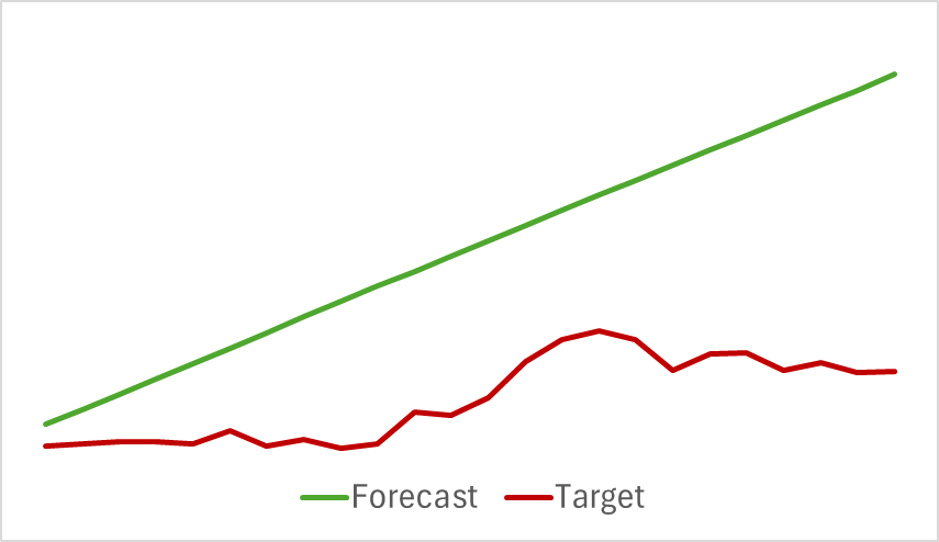
Although the predicted movement appeared linear, the digitized values still showed small fluctuations. However, these fluctuations were so minimal that they were not visualized on the graph. This raises the question: are these fluctuations enough to build a profitable strategy for our Actor?
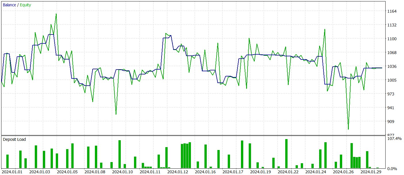
We train Actor and Critic models iteratively with periodic updates of the training dataset. As you know, periodic updates are necessary to more accurately assess the Actor's actions as its policy shifts during training.
Unfortunately, we were unable to train the Actor's policy to generate consistent profits on the testing dataset.
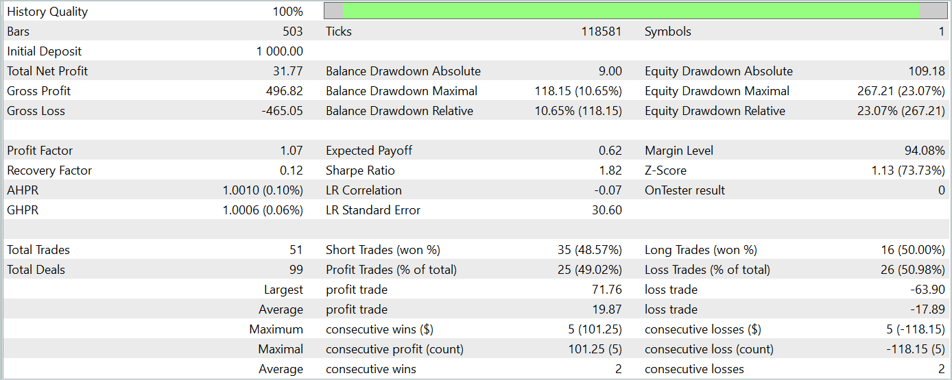
Nevertheless, we acknowledge that significant deviations from the original method's implementation were made during our work, which could have affected the results obtained.
Conclusion
In this article, we explored another approach to time series forecasting based on the spatial-temporal Transformer neural network (STNN). This model combines the advantages of the spatial-temporal information (STI) transformation equation and the Transformer structure to effectively perform multi-step forecasting of short-term time series.
STNN uses the STI equation, which transforms the spatial information of multidimensional variables into the temporal information of the target variable. This is equivalent to increasing the sample size and helps address the issue of insufficient short-term data.
To enhance the accuracy of numerical forecasting, STNN includes a continuous attention mechanism that allows the model to better focus on important aspects of the data.
In the practical part of the article, we implemented our vision of the proposed approaches in the MQL5 language. However, we made significant deviations from the original algorithm, which may have influenced the results of our experiments.
References
Programs used in the article
| # | Name | Type | Description |
|---|---|---|---|
| 1 | Research.mq5 | Expert Advisor | Example collection EA |
| 2 | ResearchRealORL.mq5 | Expert Advisor | EA for collecting examples using the Real-ORL method |
| 3 | Study.mq5 | Expert Advisor | Model training EA |
| 4 | StudyEncoder.mq5 | Expert Advisor | Encoder training EA |
| 5 | Test.mq5 | Expert Advisor | Model testing EA |
| 6 | Trajectory.mqh | Class library | System state description structure |
| 7 | NeuroNet.mqh | Class library | A library of classes for creating a neural network |
| 8 | NeuroNet.cl | Code Base | OpenCL program code library |
Translated from Russian by MetaQuotes Ltd.
Original article: https://www.mql5.com/ru/articles/15290
Warning: All rights to these materials are reserved by MetaQuotes Ltd. Copying or reprinting of these materials in whole or in part is prohibited.
This article was written by a user of the site and reflects their personal views. MetaQuotes Ltd is not responsible for the accuracy of the information presented, nor for any consequences resulting from the use of the solutions, strategies or recommendations described.

- Free trading apps
- Over 8,000 signals for copying
- Economic news for exploring financial markets
You agree to website policy and terms of use