
Neural Networks Made Easy (Part 96): Multi-Scale Feature Extraction (MSFformer)

Introduction
Time series data is widespread in the real world, playing an important role in various fields including finance. This data represents sequences of observations collected at different points in time. Deep time series analysis and modeling allow researchers to predict future trends and patterns, which is used in the decision-making process.
In recent years, many researchers have focused their efforts on studying time series using deep learning models. These methods have proven effective in capturing nonlinear relationships and handling long-term dependencies, which is especially useful for modeling complex systems. However, despite significant achievements, there are still questions of how to efficiently extract and integrate long-term dependencies and short-term features. Understanding and properly combining these two types of dependencies is critical to building accurate and reliable predictive models.
One of the options for solving this problem was presented in the paper "Time Series Prediction Based on Multi-Scale Feature Extraction". The paper presents a time series forecasting model MSFformer (Multi-Scale Feature Transformer), which is based on an improved pyramidal attention architecture. This model is designed for efficient extraction and integration of multi-scale features.
The authors of the method highlight the following innovations of MSFformer:
- Introduction of the Skip-PAM mechanism, allowing the model to effectively capture both long-term and short-term features in long time series.
- Improved CSCM module for creating pyramid data structure.
The authors of MSFformer presented experimental results on three time series datasets, which demonstrate the superior performance of the proposed model. The proposed mechanisms allow the MSFformer model process complex time series data more accurately and efficiently, ensuring high forecast accuracy and reliability.
1. The MSFformer Algorithm
The authors of the MSFformer model propose an innovative architecture of the pyramidal attention mechanism at different time intervals, which underlies their method. In addition, in order to construct multi-level temporal information in the input data, they use feature convolution in the large-scale construction module CSCM (Coarser-Scale Construction Module). This allows them to extract temporal information at a coarser level.
The CSCM module constructs a tree of features of the analyzed time series. Here, the inputs are first passed through a fully connected layer to transform the feature dimensionality to a fixed size. Then several sequential, specially designed, FCNN feature convolution blocks are used.
In the FCNN block, feature vectors are first formed by extracting data from the input sequence using a given cross-step. These vectors are then combined. The combined vectors are then subject to convolution operations. Author's visualization of the FCNN block is presented below.
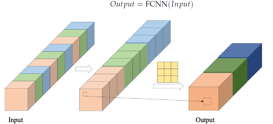
The CSCM module proposed by the authors uses several consecutive FCNN blocks. Each of them, using the results of the previous block as input, extracts features of a larger scale.
The features of different scales obtained in this way are combined into a single vector, the size of which is reduced by a linear layer to the scale of the input data.
Author's visualization of the CSCM module is presented below.
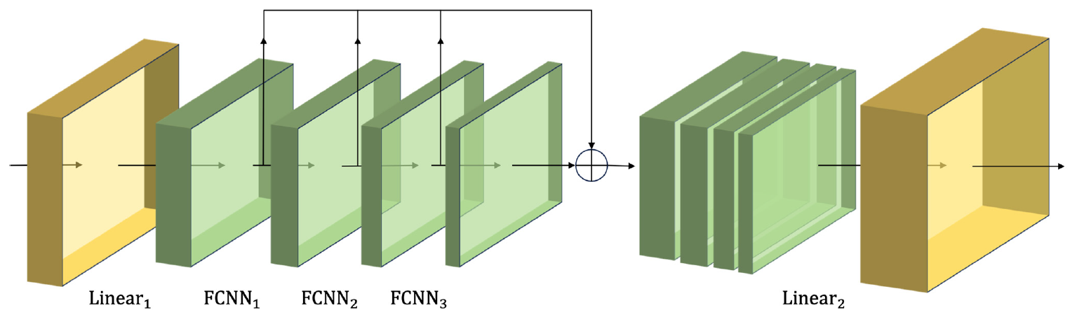
By passing the data of the analyzed time series through such CSCM, we obtain temporal information about features at different levels of granularity. We build a pyramidal tree of features by stacking FCNN layers. This allows us to the understand the data at multiple levels and provides a solid foundation for implementing the innovative pyramidal attention structure Skip-PAM (Skip-Pyramidal Attention Module).
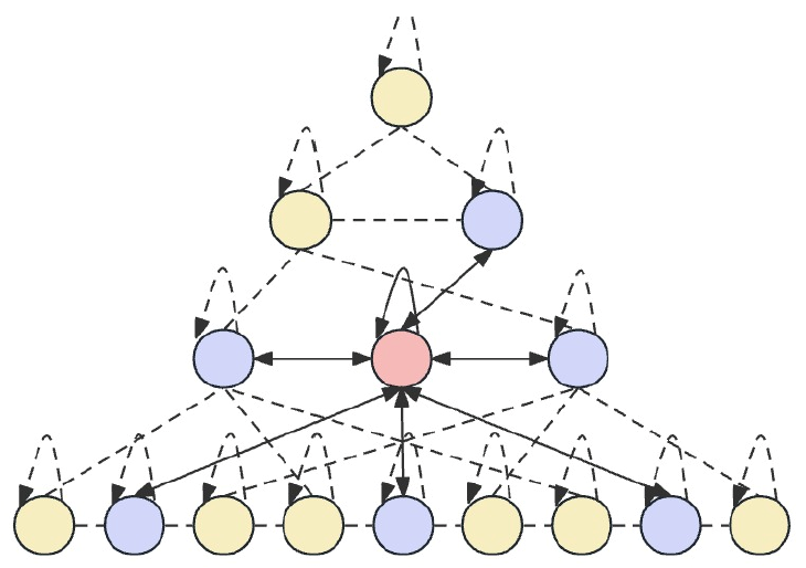
The main idea of Skip-PAM is to process the input data at different time intervals, which allows the model to capture time dependencies of different levels of granularity. At lower levels, the model may focus on short-term, detailed patterns. The upper levels are able to capture more macroscopic trends and periodicities. The proposed Skip-PAM pays more attention to periodic dependencies such as every Monday or the beginning of each month. This multi-scale approach allows the model to capture a variety of temporal relationships at different levels.
Skip-PAM extracts information from time series at multiple scales through an attention mechanism built on a temporal feature tree. This process involves intra-scale and inter-scale connections. Intra-scale connections involve performing attention computations between a node and its neighboring nodes in the same layer. Inter-scale connections involve attention computations between a node and its parent node.
Through this pyramidal attention mechanism Skip-PAM, in combination with multi-scale feature convolution in CSCM, a powerful feature extraction network is formed that can adapt to dynamic changes at different time scales, whether short-term fluctuations or long-term evolutions.
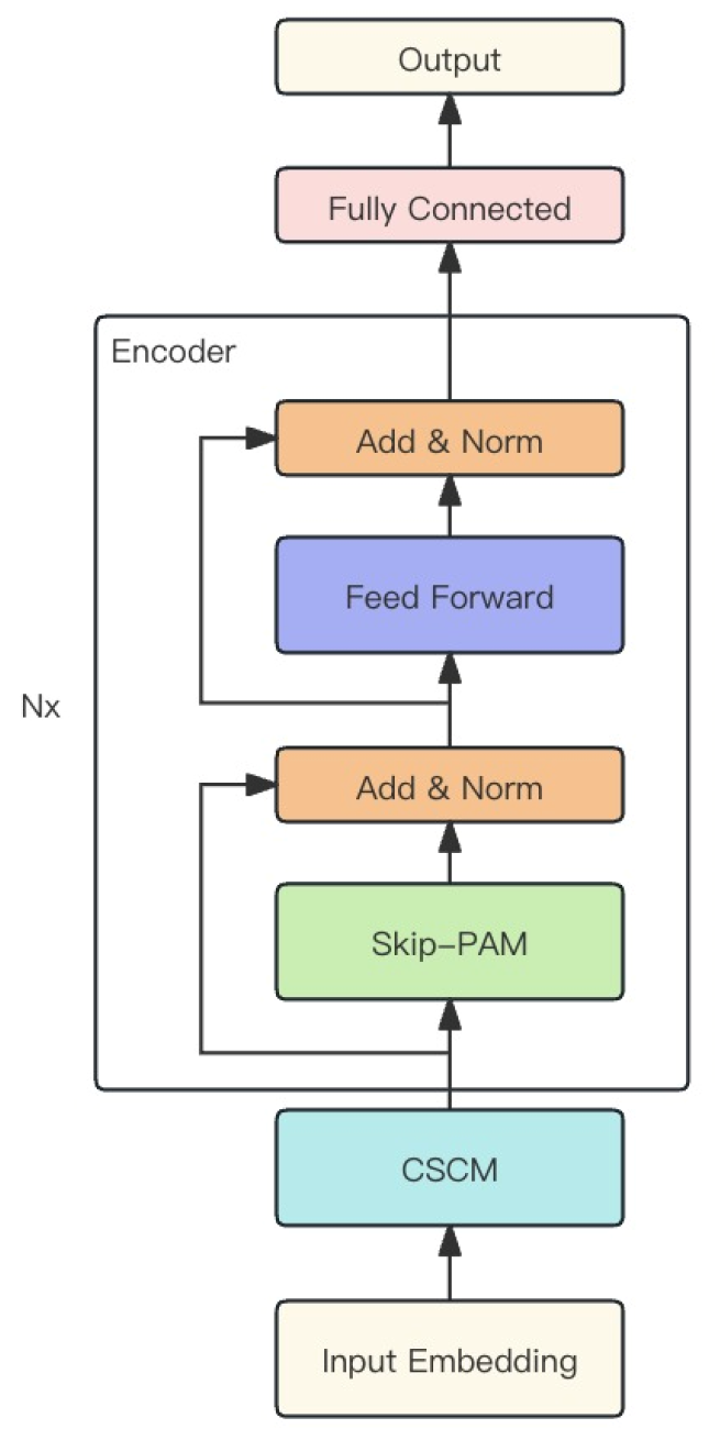
The authors of the method combine the two modules described above into one powerful MSFformer model. Its original visualization is presented below.
2. Implementing in MQL5
After considering the theoretical aspects of the MSFformer method, we move on to the practical part of our article, in which we implement our vision of the proposed approaches using MQL5.
As stated above, the proposed MSFformer method is based on 2 modules: CSCM and Skip-PAM. We will implement them within the framework of this article. There is a lot of work to be done. Let's divided it into 2 parts, in accordance with the modules being implemented.
2.1. Building the CSCM module
Let's start by building the CSCM module. To implement the architecture of this module, we will create the CNeuronCSCMOCL class, which will inherit the main functionality from the neural layer base class CNeuronBaseOCL. The structure of the new class is shown below.
class CNeuronCSCMOCL :  public CNeuronBaseOCL
  {
protected:
   uint              i_Count;
   uint              i_Variables;
   bool              b_NeedTranspose;
   //---
   CArrayInt         ia_Windows;
   CArrayObj         caTranspose;
   CArrayObj         caConvolutions;
   CArrayObj         caMLP;
   CArrayObj         caTemp;
   CArrayObj         caConvOutputs;
   CArrayObj         caConvGradients;
   //---
   virtual bool      feedForward(CNeuronBaseOCL *NeuronOCL);
   //---
   virtual bool      calcInputGradients(CNeuronBaseOCL *prevLayer);
   virtual bool      updateInputWeights(CNeuronBaseOCL *NeuronOCL);

public:
                     CNeuronCSCMOCL(void) {};
                    ~CNeuronCSCMOCL(void) {};
   virtual bool      Init(uint numOutputs, uint myIndex, COpenCLMy *open_cl,
                          uint &windows[], uint variables, uint inputs_count,
                          bool need_transpose, ENUM_OPTIMIZATION optimization_type, uint batch);
   //---
   virtual int       Type(void)   const   {  return defNeuronCSCMOCL;   }
   //---
   virtual bool      Save(int const file_handle);
   virtual bool      Load(int const file_handle);
   virtual bool      WeightsUpdate(CNeuronBaseOCL *source, float tau);
   virtual void      SetOpenCL(COpenCLMy *obj);
  };
The presented structure of the CNeuronCSCMOCL class has quite a standard set of overridable methods and a large number of dynamic arrays that will help us organize a multi-scale feature extraction structure. The purpose of dynamic arrays and declared variables will be explained during the method implementation process.
All objects of the class are declared statical. This allows us to leave the class constructor and destructor "empty". All nested objects and variables are initialized in the Init method.
As usual, in the Init method parameters, we obtain the basic constants that allow us to uniquely determine the architecture of the object being created.
In order to provide the user with the flexibility to determine the number of feature extraction layers and the size of the convolution window, we use a dynamic array windows. The number of elements in the array indicates the number of FCNN feature extraction blocks to be created. The value of each element indicates the size of the convolution window of the corresponding block.
The number of unitary time sequences in the multidimensional input time series and the size of the original sequence are specified in the variables and inputs_count parameters, respectively.
In addition, we will add a logical variable need_transpose, which will indicate the need to transpose inputs before feature extraction.
bool CNeuronCSCMOCL::Init(uint numOutputs, uint myIndex, COpenCLMy *open_cl,
                          uint &windows[], uint variables, uint inputs_count, bool need_transpose,
                          ENUM_OPTIMIZATION optimization_type, uint batch)
  {
   const uint layers = windows.Size();
   if(layers <= 0)
      return false;
   if(!CNeuronBaseOCL::Init(numOutputs, myIndex, open_cl, inputs_count * variables, optimization_type, batch))
      return false;
In the body of the method, we implement a small control block. Here we first check whether it is necessary to create at least one feature extraction block. After that, we call the method of the parent class with the same name, in which part of the control functions and initialization of inherited objects have already been implemented. We control the result of executing operations of the parent class method by the returned logical value.
In the next step, we save the received parameters into the corresponding internal variables and array.
   if(!ia_Windows.AssignArray(windows))
      return false;
   i_Variables = variables;
   i_Count = inputs_count / ia_Windows[0];
   b_NeedTranspose = need_transpose;
After that we begin the process of initializing nested objects. If there is a need to transpose the input data, we create here 2 nested data transposition layers. The first one is for transposing the input data.
   if(b_NeedTranspose)
     {
      CNeuronTransposeOCL *transp = new CNeuronTransposeOCL();
      if(!transp)
         return false;
      if(!transp.Init(0, 0, OpenCL, inputs_count, i_Variables, optimization, iBatch))
        {
         delete transp;
         return false;
        }
      if(!caTranspose.Add(transp))
        {
         delete transp;
         return false;
        }
The second one is for transposing the outputs, returning them to the dimension of the inputs.
      transp = new CNeuronTransposeOCL();
      if(!transp)
         return false;
      if(!transp.Init(0, 1, OpenCL, i_Variables, inputs_count, optimization, iBatch))
        {
         delete transp;
         return false;
        }
      if(!caTranspose.Add(transp))
        {
         delete transp;
         return false;
        }
      if(!SetOutput(transp.getOutput()) ||
         !SetGradient(transp.getGradient())
        )
         return false;
     }
Note that when we need to transpose data, we override the result and gradient buffers of our class to the corresponding buffers of the result transposition layer. This step allows us to eliminate unnecessary data copying operations.
Then we create a layer to align the size of the input data within individual unitary sequences.
   uint total = ia_Windows[0] * i_Count;
   CNeuronConvOCL *conv = new CNeuronConvOCL();
   if(!conv.Init(0, 0, OpenCL, inputs_count, inputs_count, total, 1, i_Variables, optimization, iBatch))
     {
      delete conv;
      return false;
     }
   if(!caConvolutions.Add(conv))
     {
      delete conv;
      return false;
     }
In a loop, we create the required number of convolutional feature extraction layers.
   total = 0;
   for(uint i = 0; i < layers; i++)
     {
      conv = new CNeuronConvOCL();
      if(!conv.Init(0, i + 1, OpenCL, ia_Windows[i], ia_Windows[i],
                    (i < (layers - 1) ? ia_Windows[i + 1] : 1),
                    i_Count, i_Variables, optimization, iBatch))
        {
         delete conv;
         return false;
        }
      if(!caConvolutions.Add(conv))
        {
         delete conv;
         return false;
        }
      if(!caConvOutputs.Add(conv.getOutput()) ||
         !caConvGradients.Add(conv.getGradient())
        )
         return false;
      total += conv.Neurons();
     }
Note that in the caConvolutions array, we combine the input data size alignment layer and feature extraction convolution layer. Therefore, it contains one object more than the specified number of FCNN blocks.
In accordance with the CSCM module algorithm, we need to concatenate the features of all analyzed scales into a single tensor. Therefore, along with the creation of convolution layers, we calculate the total size of the relevant output tensor. In addition, we saved pointers to the output data buffers and error gradients of the created feature extraction layers in separate dynamic arrays. This will provide faster access to their contents during model training and operation processes.
Now, having the value we need, we can create a layer to write the concatenated tensor.
   CNeuronBaseOCL *comul = new CNeuronBaseOCL();
   if(!comul.Init(0, 0, OpenCL, total, optimization, iBatch))
     {
      delete comul;
      return false;
     }
   if(!caMLP.Add(comul))
     {
      delete comul;
      return false;
     }
Here we also provide a special case for creating 1 feature extraction layer. In this case, we have nothing to combine, and the concatenated tensor will be a complete copy of the single feature extraction tensor. Therefore, to avoid unnecessary copy operations, we redefine the result and error gradient buffers.
   if(layers == 1)
     {
      comul.SetOutput(conv.getOutput());
      comul.SetGradient(conv.getGradient());
     }
After that, we create a layer for linear adjustment of the dimension of the concatenated feature tensor to the size of the input sequence.
   conv = new CNeuronConvOCL();
   if(!conv.Init(0, 0, OpenCL, total / i_Variables, total / i_Variables, inputs_count, 1,
                                                        i_Variables, optimization, iBatch))
     {
      delete conv;
      return false;
     }
   if(!caMLP.Add(conv))
     {
      delete conv;
      return false;
     }
We have overridden input and result buffers of our class for the case when we needed to transpose the input data. For a different case, we will override them now.
   if(!b_NeedTranspose)
     {
      if(!SetOutput(conv.getOutput()) ||
         !SetGradient(conv.getGradient())
        )
         return false;
     }
In this way, we eliminated unnecessary data copying operations in both cases, no matter whether the input data needs to be transposed or not.
At the end of the method, we create 3 auxiliary buffers for storing intermediate data, which we will use when concatenating features and deconcatenating the corresponding error gradients.
   CBufferFloat *buf = new CBufferFloat();
   if(!buf)
      return false;
   if(!buf.BufferInit(total, 0) || !buf.BufferCreate(OpenCL) ||
      !caTemp.Add(buf))
     {
      delete buf;
      return false;
     }
   buf = new CBufferFloat();
   if(!buf)
      return false;
   if(!buf.BufferInit(total, 0) || !buf.BufferCreate(OpenCL) ||
      !caTemp.Add(buf))
     {
      delete buf;
      return false;
     }
   buf = new CBufferFloat();
   if(!buf)
      return false;
   if(!buf.BufferInit(total, 0) || !buf.BufferCreate(OpenCL) ||
      !caTemp.Add(buf))
     {
      delete buf;
      return false;
     }
//---
   caConvOutputs.FreeMode(false);
   caConvGradients.FreeMode(false);
//---
   return true;
  }
Do not forget to control the process of creating of all nested objects. After successful initialization of all nested objects, we return the logical result of the operations to the caller.
After initializing the object of our CNeuronCSCMOCL class, we move on to creating the feed-forward algorithm. Please pay attention that within the framework of this class, we do not implement operations on the OpenCL program side. The entire implementation is based on the use of nested object methods. Their algorithm is already implemented on the OpenCL side. In such conditions, we justneed to build a high-level algorithm from the methods of nested objects and inherited from the parent class.
We organize the feed-forwad pass in the feedForward method, in the parameters of which the calling program provides a pointer to the object of the previous layer.
bool CNeuronCSCMOCL::feedForward(CNeuronBaseOCL *NeuronOCL)
  {
   CNeuronBaseOCL *inp = NeuronOCL;
   CNeuronBaseOCL *current = NULL;
In the method body, we will declare 2 variables to store pointers to neural layer objects. At this stage, we will pass the pointer received from the calling program to the source data variable. And we'll leave the second variable empty.
Next, we check the need to transpose the input data. If necessary, we perform this operation.
   if(b_NeedTranspose)
     {
      current = caTranspose.At(0);
      if(!current ||
         !current.FeedForward(inp))
         return false;
      inp = current;
     }
After that, we pass the input time series through successive convolutional feature extraction layers of different scales, whose pointers we saved in the caConvolutions array.
   int layers = caConvolutions.Total() - 1;
   for(int l = 0; l <= layers; l++)
     {
      current = caConvolutions.At(l);
      if(!current ||
         !current.FeedForward(inp))
         return false;
      inp = current;
     }
The first layer in this array is intended to align the size of the input data sequence. We do not use its result when concatenating the extracted features, which we will perform at the next stage.
Please note that we are building an algorithm without limiting the upper limit of convolutional feature extraction layers. In this case, even a minimum of 1 layer of feature extraction is allowed. And probably the simplest algorithm that we can use in this case is to create a loop with sequential addition of 1 feature array to the tensor. But this approach leads to potential multiple copying of the same data. This significantly increases our computational costs during the feed-forward pass. In order to minimize such operations, we created a branching algorithm based on the number of feature extraction blocks.
As mentioned above, there must be at least one feature extraction layer. If it is not there, then we return an error signal to the calling program in the form of a negative result.
   current = caMLP.At(0);
   if(!current)
      return false;
   switch(layers)
     {
      case 0:
         return false;
When using a single feature extraction layer, we have nothing to concatenate. As you remember, for this case, in the class initialization method we redefined the data buffers of the feature extraction and concatenation layers, which allowed us to reduce unnecessary copying operations. So, we just move on to the next operations.
      case 1:
         break;
The presence of 2 to 4 feature extraction layers leads to the choice of an appropriate data concatenation method.
      case 2:
         if(!Concat(caConvOutputs.At(0),
                    caConvOutputs.At(1),
                    current.getOutput(),
                    ia_Windows[1], 1,
                    i_Variables * i_Count))
            return false;
         break;
      case 3:
         if(!Concat(caConvOutputs.At(0),
                    caConvOutputs.At(1),
                    caConvOutputs.At(2),
                    current.getOutput(),
                    ia_Windows[1], ia_Windows[2], 1,
                    i_Variables * i_Count))
            return false;
         break;
      case 4:
         if(!Concat(caConvOutputs.At(0),
                    caConvOutputs.At(1),
                    caConvOutputs.At(2),
                    caConvOutputs.At(3),
                    current.getOutput(),
                    ia_Windows[1], ia_Windows[2], ia_Windows[3], 1,
                    i_Variables * i_Count))
            return false;
If there are more such layers, then we concatenate the first 4 feature extraction layers, but write the result to a temporary data storage buffer.
      default:
         if(!Concat(caConvOutputs.At(0),
                    caConvOutputs.At(1),
                    caConvOutputs.At(2),
                    caConvOutputs.At(3),
                    caTemp.At(0),
                    ia_Windows[1], ia_Windows[2], ia_Windows[3], ia_Windows[4],
                    i_Variables * i_Count))
            return false;
         break;
     }
Note that when performing concatenation operations, we do not access the convolutional layer objects from the caConvolutions array but directly to the buffers of their results, the pointers to which we prudently saved in the dynamic array caConvOutputs.
Next, we create a loop, starting with the 4th layer of feature extraction and stepping in 3 layers. In the body of this loop, we first calculate the size of the data window stored in the temporary buffer.
   uint last_buf = 0;
   for(int i = 4; i < layers; i += 3)
     {
      uint buf_size = 0;
      for(int j = 1; j <= i; j++)
         buf_size += ia_Windows[j];
Then we organize an algorithm for choosing a concatenation function similar to the one given above. But in this case, the temporary buffer with previously collected data will always be in first place, and the next batch of extracted features is added to it.
      switch(layers - i)
        {
         case 1:
            if(!Concat(caTemp.At(last_buf),
                       caConvOutputs.At(i),
                       current.getOutput(),
                       buf_size, 1,
                       i_Variables * i_Count))
               return false;
            break;
         case 2:
            if(!Concat(caTemp.At(last_buf),
                       caConvOutputs.At(i),
                       caConvOutputs.At(i + 1),
                       current.getOutput(),
                       buf_size, ia_Windows[i + 1], 1,
                       i_Variables * i_Count))
               return false;
            break;
         case 3:
            if(!Concat(caTemp.At(last_buf),
                       caConvOutputs.At(i),
                       caConvOutputs.At(i + 1),
                       caConvOutputs.At(i + 2),
                       current.getOutput(),
                       buf_size, ia_Windows[i + 1], ia_Windows[i + 2], 1,
                       i_Variables * i_Count))
               return false;
            break;
         default:
            if(!Concat(caTemp.At(last_buf),
                       caConvOutputs.At(i),
                       caConvOutputs.At(i + 1),
                       caConvOutputs.At(i + 2),
                       caTemp.At((last_buf + 1) % 2),
                       buf_size, ia_Windows[i + 1], ia_Windows[i + 2], ia_Windows[i + 3],
                       i_Variables * i_Count))
               return false;
            break;
        }
      last_buf = (last_buf + 1) % 2;
     }
Note that when adding the last feature layers (1 to 3), the result of the operation is saved in the data concatenation layer buffer. In other cases, we use another buffer for temporary data storage. At each iteration of the loop, the buffers are alternated in order to prevent data corruption and loss.
After concatenating all features into a single tensor, we only need to adjust the size of the result tensor.
   inp = current;
   current = caMLP.At(1);
   if(!current ||
      !current.FeedForward(inp))
      return false;
If necessary, we transpose them into the dimension of the input data.
   if(b_NeedTranspose)
     {
      inp = current;
      current = caTranspose.At(1);
      if(!current ||
         !current.FeedForward(inp))
         return false;
     }
//---
   return true;
  }
Let me remind you that in the initialization method we organized the substitution of data buffers. Therefore, the results of operations are copied into the corresponding inherited buffer of our class "automatically".
After constructing the feed-forward pass method, we move on to implementing the backpropagation algorithms. First, we create a method for propagating the error gradient to all objects, according to their influence on the overall result (calcInputGradients). As usual, in the parameters of this method we receive a pointer to the object of the previous neural layer. In this case, we need to pass on the corresponding share of the error gradient to it.
bool CNeuronCSCMOCL::calcInputGradients(CNeuronBaseOCL *prevLayer)
  {
   if(!prevLayer)
      return false;
In the body of the method, we immediately check the relevance of the received pointer. After that, we create local pointers of 2 neural layers, with which we will work sequentially.
   CNeuronBaseOCL *current = caMLP.At(0);
   CNeuronBaseOCL *next = caMLP.At(1);
Let me remind you that in the process of distributing the error gradient, we move according to the feed-forward pass algorithm, but in the opposite direction. Therefore, we first propagate the gradient through a data transposition layer, of course, if there is a need for such an operation.
   if(b_NeedTranspose)
     {
      if(!next.calcHiddenGradients(caTranspose.At(1)))
         return false;
     }
We then feed the error gradient into the concatenated layer of extracted features of different scales.
   if(!current.calcHiddenGradients(next.AsObject()))
      return false;
   next = current;
After which, we need to distribute the error gradient to the corresponding feature extraction layers.
Let's not forget about the special case of having 1 feature extraction layer. Here we only need to adjust the error gradient by the derivative of the activation function.
   int layers = caConvGradients.Total();
   if(layers == 1)
     {
      next = caConvolutions.At(1);
      if(next.Activation() != None)
        {
         if(!DeActivation(next.getOutput(), next.getGradient(), next.getGradient(), next.Activation()))
            return false;
        }
     }
In general, we first separate the error gradient of the last feature extraction layer and correct it by the derivative of the activation function.
   else
     {
      int prev_window = 0;
      for(int i = 1; i < layers; i++)
         prev_window += int(ia_Windows[i]);
      if(!DeConcat(caTemp.At(0), caConvGradients.At(layers - 1), next.getGradient(),
                                              prev_window, 1, i_Variables * i_Count))
         return false;
      next = caConvolutions.At(layers);
      int current_buf = 0;
After that, we create a reverse loop through feature extraction layers. In the body of this loop, we first obtain the error gradient from the subsequent feature extraction layer.
      for(int l = layers; l > 1; l--)
        {
         current = caConvolutions.At(l - 1);
         if(!current.calcHiddenGradients(next.AsObject()))
            return false;
Then we extract the fraction of the analyzed layer from the buffer of error gradients of the concatenated feature tensor.
         int window = int(ia_Windows[l - 1]);
         prev_window -= window;
         if(!DeConcat(caTemp.At((current_buf + 1) % 2), caTemp.At(2), caTemp.At(current_buf),
                                                  prev_window, window, i_Variables * i_Count))
            return false;
We adjust it for the derivative of the activation function.
         if(current.Activation() != None)
           {
            if(!DeActivation(current.getOutput(), caTemp.At(2), caTemp.At(2), current.Activation()))
               return false;
           }
And we sum up the error gradients from the 2 data streams.
         if(!SumAndNormilize(current.getGradient(), caTemp.At(2), current.getGradient(), 1, false, 0, 0, 0, 1))
            return false;
         next = current;
         current_buf = (current_buf + 1) % 2;
        }
     }
After that, we move on to the next iteration of our loop.
This way, we distribute the error gradient across all feature extraction layers. Then we pass the error gradient to the input data size alignment layer.
   current = caConvolutions.At(0);
   if(!current.calcHiddenGradients(next.AsObject()))
      return false;
   next = current;
If necessary, we propagate the error gradient through a data transposition layer.
   if(b_NeedTranspose)
     {
      current = caTranspose.At(0);
      if(!current.calcHiddenGradients(next.AsObject()))
         return false;
      next = current;
     }
At the end of the method operations, we pass the error gradient to the previous neural layer, the pointer to which we received in the parameters of this method.
   if(!prevLayer.calcHiddenGradients(next.AsObject()))
      return false;
//---
   return true;
  }
As you know, the error gradient propagation is not the goal of model training. It is only a means to determine the direction and extent of adjustment of the model parameters. Therefore, after successfully propagating the error gradient, we have to adjust the model parameters in such a way as to minimize the overall error of its operation. This functionality is implemented in the updateInputWeights method.
bool CNeuronCSCMOCL::updateInputWeights(CNeuronBaseOCL *NeuronOCL)
  {
   CObject *prev = (b_NeedTranspose ? caTranspose.At(0) : NeuronOCL);
   CNeuronBaseOCL *current = NULL;
In the method parameters, as before, we receive a pointer to the object of the previous neural layer. However, in this case we do not check the relevance of the received index. We just save it to a local variable. There is a nuance here, though. The data transposition layer does not contain any parameters. Therefore, we do not call the model parameter adjustment method for it. But for the input size alignment layer, we will select the previous layer depending on the b_NeedTranspose parameter, which indicates whether the input data needs to be transposed.
Next, we organize a loop of sequential adjustment of the parameters of the convolutional layers, including a layer for adjusting the size of the original sequence and feature extraction blocks.
   for(int i = 0; i < caConvolutions.Total(); i++)
     {
      current = caConvolutions.At(1);
      if(!current ||
         !current.UpdateInputWeights(prev)
        )
         return false;
      prev = current;
     }
Next we need to adjust the parameters of the result size aligning layer.
   current = caMLP.At(1);
   if(!current ||
      !current.UpdateInputWeights(caMLP.At(0))
     )
      return false;
//---
   return true;
  }
Other nested objects of our CNeuronCSCMOCL class do not contain trainable parameters.
At this point, the implementation of the CSCM module's main algorithms can be considered complete. Of course, the functionality of our class will not be complete without additional implementation of auxiliary method algorithms. But in order to reduce the volume of the article, I will not provide their descriptions here. You will find the complete code for all methods of this class in the attachment. The attachment also contains complete code for all programs used in the article. And we move on to building the algorithms of the next module - Skip-PAM.
2.2 Implementing Skip-PAM module algorithms
The second part of the work we have to do is to implement the pyramidal attention algorithm. The innovation of the MSFformer method authors is the application of attention algorithms to a feature tree with different intervals. The authors of the method use fixed steps between features within one level of attention. In our implementation, we will proceed a little differently. What if we let the model learn on its own which features each individual attention pyramid will analyze at each individual attention level? Sounds promising. Also, the implementation, in my opinion, is obvious and simple. We'll just add a S3 layer before each attention level.
We will build algorithms for our Skip-PAM module implementation within the CNeuronSPyrAttentionOCL class. Its structure is presented below.
class CNeuronSPyrAttentionOCL :  public CNeuronBaseOCL
  {
protected:
   uint              iWindowIn;
   uint              iWindowKey;
   uint              iHeads;
   uint              iHeadsKV;
   uint              iCount;
   uint              iPAMLayers;
   //---
   CArrayObj         caS3;
   CArrayObj         caQuery;
   CArrayObj         caKV;
   CArrayInt         caScore;
   CArrayObj         caAttentionOut;
   CArrayObj         caW0;
   CNeuronConvOCL    cFF1;
   CNeuronConvOCL    cFF2;
   //---
   virtual bool      feedForward(CNeuronBaseOCL *NeuronOCL);
   virtual bool      AttentionOut(CBufferFloat *q, CBufferFloat *kv, int scores, CBufferFloat *out, int window);
   virtual bool      AttentionInsideGradients(CBufferFloat *q, CBufferFloat *q_g, CBufferFloat *kv,
                                              CBufferFloat *kv_g, int scores, CBufferFloat *gradient);
   //---
   virtual bool      calcInputGradients(CNeuronBaseOCL *prevLayer);
   virtual bool      updateInputWeights(CNeuronBaseOCL *NeuronOCL);
   virtual void      ArraySetOpenCL(CArrayObj *array, COpenCLMy *obj);

public:
                     CNeuronSPyrAttentionOCL(void) {};
                    ~CNeuronSPyrAttentionOCL(void) {};
   virtual bool      Init(uint numOutputs, uint myIndex, COpenCLMy *open_cl,
                          uint window_in, uint window_key, uint heads, uint heads_kv,
                          uint units_count, uint pam_layers,
                          ENUM_OPTIMIZATION optimization_type, uint batch);
   //---
   virtual int       Type(void)   const   {  return defNeuronSPyrAttentionMLKV;   }
   //---
   virtual bool      Save(int const file_handle);
   virtual bool      Load(int const file_handle);
   virtual bool      WeightsUpdate(CNeuronBaseOCL *source, float tau);
   virtual void      SetOpenCL(COpenCLMy *obj);
  };
As you can see from the presented structure, the new class contains even more dynamic arrays and parameters. Their names are in line with objects of other attention classes. As you understand, this is done on purpose. We will get acquainted with the use of created objects and variables during the implementation process.
As before, we begin our consideration of the algorithms of the new class with the object Init initialization method.
bool CNeuronSPyrAttentionOCL::Init(uint numOutputs, uint myIndex, COpenCLMy *open_cl,
                                   uint window_in, uint window_key, uint heads,
                                   uint heads_kv, uint units_count, uint pam_layers,
                                   ENUM_OPTIMIZATION optimization_type, uint batch)
  {
   if(!CNeuronBaseOCL::Init(numOutputs, myIndex, open_cl, window_in * units_count, optimization_type, batch))
      return false;
In the method parameters, we receive the main constants that determine the architecture of he object being created. In the body of the method, we call the relevant method of the parent class, in which the minimum necessary controls and initialization of inherited objects are implemented.
It should also be noted that within the framework of this method, we will analyze individual time steps within the overall multimodal time sequence. However, in this case, it is probably difficult to refer to the original data input to the Skip-PAM module as multimodal time series. Because the results of the previous CSCM module represent a set of extracted features of different data scales, rather than a time sequence.
After successful execution of the initialization method of the parent class objects, we save the obtained constants in local variables.
   iWindowIn = window_in;
   iWindowKey = MathMax(window_key, 1);
   iHeads = MathMax(heads, 1);
   iHeadsKV = MathMax(heads_kv, 1);
   iCount = units_count;
   iPAMLayers = MathMax(pam_layers, 2);
Pay attention to the appearance of a new parameter iPAMLayers, which determines the number of levels of pyramidal attention. The remaining parameters imply the same functionality as the attention methods discussed earlier. We have also preserved the iHeadsKV parameter for the possibility of using the number of Key-Value heads different from the dimensions of the Query attention heads, as it was considered in the MLKV method.
Then we clear the dynamic arrays.
   caS3.Clear();
   caQuery.Clear();
   caKV.Clear();
   caScore.Clear();
   caAttentionOut.Clear();
   caW0.Clear();
Let's create the necessary local variables.
   CNeuronBaseOCL *base = NULL;
   CNeuronConvOCL *conv = NULL;
   CNeuronS3      *s3 = NULL;
We create the initialization loop for the pyramidal attention block objects. As you might guess, the number of iterations of the loop is equal to the number of attention levels created.
   for(uint l = 0; l < iPAMLayers; l++)
     {
      //--- S3
      s3 = new CNeuronS3();
      if(!s3)
         return false;
      if(!s3.Init(0, l, OpenCL, iWindowIn, iCount, optimization, iBatch) ||
         !caS3.Add(s3))
         return false;
      s3.SetActivationFunction(None);
In the body of the loop we first create the S3 layer, in which the permutation of the analyzed sequence is organized. In this case, we use only one data mixing layer with a window equal to the number of analyzed parameters in the original multimodal sequence.
Then we create Query, Key and Value entity generation objects. Please note that when forming entities, we use one INPUT data object, but different attention head parameters.
      //--- Query
      conv = new CNeuronConvOCL();
      if(!conv)
         return false;
      if(!conv.Init(0, 0, OpenCL, iWindowIn, iWindowIn, iWindowKey*iHeads, iCount, optimization, iBatch) ||
         !caQuery.Add(conv))
        {
         delete conv;
         return false;
        }
      conv.SetActivationFunction(None);
      //--- KV
      conv = new CNeuronConvOCL();
      if(!conv)
         return false;
      if(!conv.Init(0, 0, OpenCL, iWindowIn, iWindowIn, 2*iWindowKey*iHeadsKV, iCount, optimization, iBatch) ||
         !caKV.Add(conv))
        {
         delete conv;
         return false;
        }
      conv.SetActivationFunction(None);
We will create the matrix of dependence coefficients only on the OpenCL context side. Here we will only save a pointer to the buffer.
      //--- Score
      int temp = OpenCL.AddBuffer(sizeof(float) * iCount * iCount * iHeads, CL_MEM_READ_WRITE);
      if(temp < 0)
         return false;
      if(!caScore.Add(temp))
         return false;
In the next step, we create a layer to record the results of multi-headed attention.
      //--- MH Attention Out
      base = new CNeuronBaseOCL();
      if(!base)
         return false;
      if(!base.Init(0, 0, OpenCL, iWindowKey * iHeadsKV * iCount, optimization, iBatch) ||
         !caAttentionOut.Add(conv))
        {
         delete base;
         return false;
        }
      base.SetActivationFunction(None);
The iterations of the loop are completed by a layer of dimensionality reduction down to the input data level.
      //--- W0
      conv = new CNeuronConvOCL();
      if(!conv)
         return false;
      if(!conv.Init(0, 0, OpenCL, iWindowKey * iHeadsKV, iWindowKey * iHeadsKV, iWindowIn, iCount,
                                                                              optimization, iBatch) ||
         !caW0.Add(conv))
        {
         delete conv;
         return false;
        }
      conv.SetActivationFunction(None);
     }
After successful completion of all iterations of creating pyramidal attention levels, we add a layer. In the buffer of this layer we will record the sum of the results of the pyramidal attention block and the input data.
//--- Residual
   base = new CNeuronBaseOCL();
   if(!base)
      return false;
   if(!base.Init(0, 0, OpenCL, iWindowIn * iCount, optimization, iBatch) ||
      !caW0.Add(conv))
     {
      delete base;
      return false;
     }
   base.SetActivationFunction(None);
Now we just need to initialize the FeedForward block layers.
//--- FeedForward
   if(!cFF1.Init(0, 0, OpenCL, iWindowIn, iWindowIn, 4 * iWindowIn, iCount, optimization, iBatch))
      return false;
   cFF1.SetActivationFunction(LReLU);
   if(!cFF2.Init(0, 0, OpenCL, 4 * iWindowIn, 4 * iWindowIn, iWindowIn, iCount, optimization, iBatch))
      return false;
   cFF2.SetActivationFunction(None);
   if(!SetGradient(cFF2.getGradient()))
      return false;
Ahe end of the method, we forcefully remove the activation function of our layer.
   SetActivationFunction(None);
//---
   return true;
  }
After initializing the objects of our class, we move on to implementing the feed-forward pass algorithms. Here we need to do a little preparatory work on the OpenCL program side. We will create a new MH2PyrAttentionOut kernel, which is essentially a modified version of the MH2AttentionOut kernel.
__kernel void MH2PyrAttentionOut(__global float *q,
                                 __global float *kv,
                                 __global float *score,
                                 __global float *out,
                                 const int dimension,
                                 const int heads_kv,
                                 const int window
                                )
  {
//--- init
   const int q_id = get_global_id(0);
   const int k = get_global_id(1);
   const int h = get_global_id(2);
   const int qunits = get_global_size(0);
   const int kunits = get_global_size(1);
   const int heads = get_global_size(2);
In addition to the kernel name, it differs from the previous one by the presence of an additional window parameter for the attention window. We plan to call the kernel in a 3-dimensional task space. As always, at the beginning of the kernel we identify thread in all dimensions of the task space.
Next, we calculate the necessary constants.
   const int h_kv = h % heads_kv;
   const int shift_q = dimension * (q_id * heads + h);
   const int shift_k = dimension * (2 *  heads_kv * k + h_kv);
   const int shift_v = dimension * (2 *  heads_kv * k + heads_kv + h_kv);
   const int shift_s = kunits * (q_id *  heads + h) + k;
   const uint ls = min((uint)get_local_size(1), (uint)LOCAL_ARRAY_SIZE);
   const int delta_win = (window + 1) / 2;
   float koef = sqrt((float)dimension);
   if(koef < 1)
      koef = 1;
We also initialize a local array to record intermediate values.
__local float temp[LOCAL_ARRAY_SIZE];
First, we need to determine the dependency coefficients for each element of the sequence. As you know, in the attention block, the dependence coefficients are normalized by the SoftMax function. For this, we first calculate the sum of the exponents of the dependence coefficients.
In the first stage, each thread will collect its part of the sum of exponential values into the corresponding element of the local data array. Please note the following addition: we calculate the dependence coefficients only within the attention window of the current element. For all other elements, the dependence coefficient is "0".
//--- sum of exp
   uint count = 0;
   if(k < ls)
      do
        {
         if((count * ls) < (kunits - k))
           {
            float sum = 0;
            if(abs(count * ls + k - q_id) <= delta_win)
              {
               for(int d = 0; d < dimension; d++)
                  sum = q[shift_q + d] * kv[shift_k + d];
               sum = exp(sum / koef);
               if(isnan(sum))
                  sum = 0;
              }
            temp[k] = (count > 0 ? temp[k] : 0) + sum;
           }
         count++;
        }
      while((count * ls + k) < kunits);
   barrier(CLK_LOCAL_MEM_FENCE);
To synchronize local group threads, we use a barrier.
In the next step, we need to collect the sum of the values of all elements of the local array. For this, we create another loop, in which we synchronize local threads at each iteration. Here you need to be careful that each thread visits the same number of barriers. Otherwise, we may get "freezing" of individual threads.
   count = min(ls, (uint)kunits);
//---
   do
     {
      count = (count + 1) / 2;
      if(k < ls)
         temp[k] += (k < count && (k + count) < kunits ? temp[k + count] : 0);
      if(k + count < ls)
         temp[k + count] = 0;
      barrier(CLK_LOCAL_MEM_FENCE);
     }
   while(count > 1);
After determining the sum of the exponents, we can calculate the normalized dependence coefficients. Do not forget that dependencies are only present within the attention window.
//--- score
   float sum = temp[0];
   float sc = 0;
   if(sum != 0 && abs(k - q_id) <= delta_win)
     {
      for(int d = 0; d < dimension; d++)
         sc = q[shift_q + d] * kv[shift_k + d];
      sc = exp(sc / koef) / sum;
      if(isnan(sc))
         sc = 0;
     }
   score[shift_s] = sc;
   barrier(CLK_LOCAL_MEM_FENCE);
Of course, we synchronize local threads after calculating dependency coefficients.
Next, we need to determine the value of the elements taking into account dependencies. Here we will use the same algorithm for summing values in parallel threads as we did when determining the sum of exponential values of dependencies. We first collect the sums of the individual values in the elements of the local array.
//--- out
   for(int d = 0; d < dimension; d++)
     {
      uint count = 0;
      if(k < ls)
         do
           {
            if((count * ls) < (kunits - k))
              {
               float sum = 0;
               if(abs(count * ls + k - q_id) <= delta_win)
                 {
                  sum = kv[shift_v + d] * (count == 0 ? sc : score[shift_s + count * ls]);
                  if(isnan(sum))
                     sum = 0;
                 }
               temp[k] = (count > 0 ? temp[k] : 0) + sum;
              }
            count++;
           }
         while((count * ls + k) < kunits);
      barrier(CLK_LOCAL_MEM_FENCE);
And then we collect the sum of the values of the array elements.
      //---
      count = min(ls, (uint)kunits);
      do
        {
         count = (count + 1) / 2;
         if(k < ls)
            temp[k] += (k < count && (k + count) < kunits ? temp[k + count] : 0);
         if(k + count < ls)
            temp[k + count] = 0;
         barrier(CLK_LOCAL_MEM_FENCE);
        }
      while(count > 1);
      //---
      out[shift_q + d] = temp[0];
     }
  }
We save the resulting sum in the corresponding element of the result buffer.
Thus, we have created a new attention kernel within the given window. Please note that for elements outside the attention window we have set the dependency coefficients to "0". This simple move allows us to use the previously created MH2AttentionInsideGradients kernel to distribute the error gradient within the backpropagation pass.
To place the specified kernels in the execution queue on the main program side, I have created the AttentionOut and AttentionInsideGradients methods, respectively. Their algorithm does not differ much from similar methods discussed in previous articles within this series, so we will not dwell on them in detail now. You can find the code them yourself in the attachment. And we move on to the implementation of the feedForward method algorithms.
In the parameters, the forward pass method receives a pointer to the object of the previous neural layer, which contains the input data.
bool CNeuronSPyrAttentionOCL::feedForward(CNeuronBaseOCL *NeuronOCL)
  {
   CNeuronBaseOCL *prev = NeuronOCL;
   CNeuronBaseOCL *current = NULL;
   CBufferFloat   *q = NULL;
   CBufferFloat   *kv = NULL;
In the body of the method, we create a number of local variables to store pointers to the processed objects of the nested neural layers.
Next, we create a loop through the attention levels. In the body of the loop, we first shuffle the source data.
   for(uint l = 0; l < iPAMLayers; l++)
     {
      //--- Mix
      current = caS3.At(l);
      if(!current ||
         !current.FeedForward(prev.AsObject())
        )
         return false;
      prev = current;
After that we generate tensors of the Query, Key and Value entities to implement the multi-headed attention algorithm.
      //--- Query
      current = caQuery.At(l);
      if(!current ||
         !current.FeedForward(prev.AsObject())
        )
         return false;
      q = current.getOutput();
      //--- Key and Value
      current = caKV.At(l);
      if(!current ||
         !current.FeedForward(prev.AsObject())
        )
         return false;
      kv = current.getOutput();
Execute the attention kernel algorithm for this level.
      //--- PAM
      current = caAttentionOut.At(l);
      if(!current || !AttentionOut(q, kv, caScore.At(l), current.getOutput(), iPAMLayers - l))
         return false;
      prev = current;
Note that at each subsequent level, we reduce the attention window, thereby creating a pyramid effect. For this we use the difference "iPAMLayers - l".
At the end of the loop iterations, we reduce the size of the multi-headed attention result tensor down to the the input data size.
      //--- W0
      current = caW0.At(l);
      if(!current ||
         !current.FeedForward(prev.AsObject())
        )
         return false;
      prev = current;
     }
After successfully completing all levels of pyramidal attention, we sum and normalize the results of attention with the input data.
//--- Residual
   current = caW0.At(iPAMLayers);
   if(!SumAndNormilize(NeuronOCL.getOutput(), prev.getOutput(), current.getOutput(), iWindowIn, true))
      return false;
And the last one in the pyramidal attention layer is the FeedForward block, similar to the vanilla Transformer.
//---FeedForward
   if(!cFF1.FeedForward(current.AsObject()) ||
      !cFF2.FeedForward(cFF1.AsObject())
     )
      return false;
We then sum and normalize the data from the 2 threads again.
//--- Residual
   if(!SumAndNormilize(current.getOutput(), cFF2.getOutput(), getOutput(), iWindowIn, true))
      return false;
//---
   return true;
  }
Remember to control the execution of operations. At the end of the method, we return the logical result of the operations to the caller.
As usual, after implementing the feed-forward pass, we move on to constructing the backpropagation pass algorithms, which consists of 2 stages: propagation of the error gradient and optimization of the model parameters.
The propagation of error gradients is implemented in the calcInputGradients method.
bool CNeuronSPyrAttentionOCL::calcInputGradients(CNeuronBaseOCL *prevLayer)
  {
   if(!prevLayer)
      return false;
In the parameters of this method, we receive a pointer to the object of the previous neural layer. Into the buffer of this layer, we must transfer the error gradient in accordance with the influence of the input data on the overall result.
Next, we create some local variables to temporarily store pointers to internal objects.
   CNeuronBaseOCL *next = NULL;
   CNeuronBaseOCL *current = NULL;
   CNeuronBaseOCL *q = NULL;
   CNeuronBaseOCL *kv = NULL;
The distribution of error gradients is performed in accordance with the feed-forward pass operations, but in reverse order. First, we propagate the error gradient through the FeedForward block.
//--- FeedForward
   current = caW0.At(iPAMLayers);
   if(!current ||
      !cFF1.calcHiddenGradients(cFF2.AsObject()) ||
      !current.calcHiddenGradients(cFF1.AsObject())
     )
      return false;
   next = current;
Then we need to add the error gradients from the 2 operation threads.
//--- Residual
   current = caW0.At(iPAMLayers - 1);
   if(!SumAndNormilize(getGradient(), next.getGradient(), current.getGradient(), iWindowIn, false))
      return false;
   CBufferFloat *residual = next.getGradient();
   next = current;
After that, we create a reverse loop through the attention levels with a sequential error gradient descent.
   for(int l = int(iPAMLayers - 1); l >= 0; l--)
     {
      //--- W0
      current = caAttentionOut.At(l);
      if(!current ||
         !current.calcHiddenGradients(next.AsObject())
        )
         return false;
In the body of the loop, we first propagate the error gradient across the attention heads. Then we propagate it down to the Query, Key and Value entity level.
      //--- MH Attention
      q = caQuery.At(l);
      kv = caKV.At(l);
      if(!q || !kv ||
         !AttentionInsideGradients(q.getOutput(), q.getGradient(), kv.getOutput(), kv.getGradient(),
                                                                   caScore.At(l), current.getGradient())
        )
         return false;
The next step is to propagate the error gradient down to the data shuffling layer. Here, we need to combine data from 2 threads - Query and Key-Value. To do this, we first obtain the error gradient from Query and transfer it to a temporary buffer.
      //--- Query
      current = caS3.At(l);
      if(!current ||
         !current.calcHiddenGradients(q.AsObject()) ||
         !Concat(current.getGradient(), current.getGradient(), residual, iWindowIn,0, iCount)
        )
         return false;
Then we take the gradient from Key-Value and sum the results of the 2 data threads.
      //--- Key and Value
      if(!current ||
         !current.calcHiddenGradients(kv.AsObject()) ||
         !SumAndNormilize(current.getGradient(), residual, current.getGradient(), iWindowIn, false)
        )
         return false;
      next = current;
We propagate the error gradient through the data shuffling layer and move on to the next iteration of the loop.
      //--- S3
      current = (l == 0 ? prevLayer : caW0.At(l - 1));
      if(!current ||
         !current.calcHiddenGradients(next.AsObject())
        )
         return false;
      next = current;
     }
At the end of the method operations, we just need to combine the error gradient from the two threads. Here we first adjust the error gradient of the residual connections by the derivative of the activation function of the previous layer. When the error gradient descends directly to the layer level, the adjustment of the error gradient to the activation function occurs automatically.
   current = caW0.At(iPAMLayers - 1);
   if(!DeActivation(prevLayer.getOutput(), current.getGradient(), residual, prevLayer.Activation()) ||
      !SumAndNormilize(prevLayer.getGradient(), residual, prevLayer.getGradient(), iWindowIn, false)
     )
      return false;
//---
   return true;
  }
And then we sum the error gradients from both threads.
After distributing the error gradients, we move on to adjusting the model parameters. We implement this functionality in the updateInputWeights method. The algorithm of this method is quite straightforward - we sequentially call the same-name methods of nested objects that contain the learnable parameters.
bool CNeuronSPyrAttentionOCL::updateInputWeights(CNeuronBaseOCL *NeuronOCL)
  {
   CNeuronBaseOCL *prev = NeuronOCL;
   CNeuronBaseOCL *current = NULL;
   for(uint l = 0; l < iPAMLayers; l++)
     {
      //--- S3
      current = caS3.At(l);
      if(!current ||
         !current.UpdateInputWeights(prev)
        )
         return false;
      //--- Query
      prev = current;
      current = caQuery.At(l);
      if(!current ||
         !current.UpdateInputWeights(prev)
        )
         return false;
      //--- Key and Value
      current = caKV.At(l);
      if(!current ||
         !current.UpdateInputWeights(prev)
        )
         return false;
      //--- W0
      prev = caAttentionOut.At(l);
      current = caW0.At(l);
      if(!current ||
         !current.UpdateInputWeights(prev)
        )
         return false;
      prev = current;
     }
//--- FeedForward
   prev = caW0.At(iPAMLayers);
   if(!cFF1.UpdateInputWeights(prev) ||
      !cFF2.UpdateInputWeights(cFF1.AsObject())
     )
      return false;
//---
   return true;
  }
Make sure to control the process of executing all operations of the method and return the logical result of the performed operations to the caller.
This concludes our work on implementing the proposed approaches of the MSFformer method. You can see the full code of the created classes and their methods in the attachment.
Conclusion
In this article, we have considered another interesting and promising method for forecasting time series: MSFformer (Multi-Scale Feature Transformer). The method was first presented in the paper "Time Series Prediction Based on Multi-Scale Feature Extraction". The proposed algorithm is based on an improved pyramidal attention architecture and a new approach to multi-scale feature extraction of different scales from the input data.
In the practical part of the article, we implemented 2 main modules of the proposed algorithm. We will look at the results of this work in the next article.
References
Programs used in the article
| # | Name | Type | Description |
|---|---|---|---|
| 1 | Research.mq5 | EA | Example collection EA |
| 2 | ResearchRealORL.mq5 | EA | EA for collecting examples using the Real-ORL method |
| 3 | Study.mq5 | EA | Model training EA |
| 4 | StudyEncoder.mq5 | EA | Encoder training EA |
| 5 | Test.mq5 | EA | Model testing EA |
| 6 | Trajectory.mqh | Class library | System state description structure |
| 7 | NeuroNet.mqh | Class library | A library of classes for creating a neural network |
| 8 | NeuroNet.cl | Code Base | OpenCL program code library |
Translated from Russian by MetaQuotes Ltd.
Original article: https://www.mql5.com/ru/articles/15156
Warning: All rights to these materials are reserved by MetaQuotes Ltd. Copying or reprinting of these materials in whole or in part is prohibited.
This article was written by a user of the site and reflects their personal views. MetaQuotes Ltd is not responsible for the accuracy of the information presented, nor for any consequences resulting from the use of the solutions, strategies or recommendations described.

- Free trading apps
- Over 8,000 signals for copying
- Economic news for exploring financial markets
You agree to website policy and terms of use