Chaos theory in trading (Part 1): Introduction, application in financial markets and Lyapunov exponent

Introduction to chaos theory and its relation to financial markets

What is chaos theory and how can it be applied to financial markets? We will deal with this issue in the article.

I am going to write a series of articles that will answer the questions what chaos theory is and how the concept of chaos in the market, proposed by Bill Williams, differs from the conventional, scientifically based theory. How does the theory describe the market? How and in what areas of trading can it be applied? 

We will analyze both the theoretical basis and create a number of tools that can help traders in trading.

Basic concepts of chaos theory: Attractors, fractals, and the butterfly effect

Chaos theory is an interesting field of mathematics and physics that helps us better understand complex systems, such as financial markets. Let's look at the three main ideas of this theory:

1. Attractors: These are like magnets for the states of the system - the system gravitates towards them over time. In financial markets, these may be specific prices or repeating patterns that the market returns to again and again. Strange attractors, that can be found in chaotic systems, are of particular interest. They look complex and can reveal hidden order in the random behavior of the market.

2. Fractals: These are geometric shapes that look the same at any level of magnification. In financial markets, fractals can be seen in price charts - the same pattern can be seen on both short and long timeframes. This allows the same analysis methods to be applied across different time intervals, helping to analyze price changes and assess risks.

3. Butterfly effect: This effect shows that even the smallest changes at the start can lead to large and unexpected consequences. In the world of finance, this means that small changes in the data or in the model can change the forecasts dramatically. This makes long-term forecasting in financial markets challenging and highlights the importance of continually updating and adapting our models to new conditions.

Understanding these ideas helps analysts and traders look at markets in a new way, discovering hidden patterns and possible entry or exit points for trades. Chaos theory opens up new avenues for analysis and prediction that go beyond conventional models.

Chaotic systems in the context of financial markets

Financial markets have characteristics of chaotic systems, which is important for their analysis and forecasting.

• Non-linearity: Small changes cause disproportionate fluctuations.
• Sensitivity to initial conditions: Small events can lead to big movements.
• Self-organization: Formation of trends and patterns without external control.
• Fractal structure: Price charts exhibit fractal properties.
• Limited predictability: Forecast accuracy decreases with increasing horizon.
• Strange attractors: Fluctuations around certain levels or states.
• Transitions between states: Sudden transitions from stability to volatility.

Understanding this helps in developing sophisticated analysis methods, risk management and trading algorithms.

Volatility in trading

Volatility is a key concept in trading and finance, related to chaos theory. It measures how much the price of an asset changes over a given period of time. In trading, volatility helps assess risk, price options and develop trading strategies.

Financial markets often behave like chaotic systems. They can react unexpectedly to small changes, similar to the butterfly effect. Markets can also self-organize, creating trends and patterns without outside intervention, and price charts show similarities across different timeframes, which are called fractal properties.

Chaos theory offers unique tools for volatility analysis, such as phase space reconstruction and the Lyapunov exponent, which help find hidden patterns and assess predictability. These chaotic models can complement traditional methods such as GARCH models, particularly in identifying market regimes and predicting abrupt changes in volatility.

Understanding the chaotic nature of volatility opens up new opportunities for more accurate analysis and forecasting of market dynamics, which leads to the development of efficient trading strategies and risk management methods.

Conventional chaos theory and Bill Williams' approach

Conventional chaos theory and Bill Williams' concept of "chaos" are very different. The former relies on rigorous mathematical principles and uses sophisticated tools to analyze systems. The latter, on the other hand, uses an intuitive approach and technical indicators, such as Alligator and Fractals, which have no direct connection to the mathematical theory of chaos.

Conventional chaos theory is based on rigorous mathematical principles and scientific research in the field of non-linear dynamics. It uses rigorous mathematical methods and considers chaos to exhibit deterministic but unpredictable behavior. Williams uses the term "chaos" more loosely, referring to the general unpredictability of markets. His methods are aimed at practical application in trading, rather than at deep analysis of the chaotic nature of the markets.

Although Williams adapted some terms from chaos theory, his approach is based more on technical analysis and personal interpretation of market movements. This has drawn criticism from chaos theorists, who find the use of the term "chaos" in this context misleading.

Chaos theory in market analysis

Chaos theory offers a new perspective on the analysis of market dynamics, recognizing the complexity and unpredictability of financial markets. Unlike traditional methods, chaos theory takes into account the non-linearity and complexity of market processes.

This approach helps explain why small events can lead to large market movements, and why long-term forecasts are often inaccurate. Chaos theory allows us to analyze phenomena such as market crashes and bubbles, providing new tools for more accurate and adaptive market analysis.

Lyapunov exponent and its application in financial time series analysis

The Lyapunov exponent is a tool from chaos theory that helps us understand how sensitive a system is to initial conditions. In financial markets, this is important because it allows one to estimate how much prices will change with small changes in market conditions.

If the Lyapunov exponent is positive, it means that the system behaves chaotically: small changes can lead to large fluctuations in the future. If the exponent is negative, the system is more stable and prices will change less.

Using this exponent, you can determine when the market becomes more volatile and predictable. High values may indicate possible sharp price changes, which is useful for assessing risk and adjusting trading strategies.

To calculate the Lyapunov exponent in financial data, it is necessary to create a phase space by analyzing how close points in this space diverge. This process requires choosing the right parameters, such as dimension and time delay.

One important aspect of using the Lyapunov exponent is to estimate how long forecasts will be accurate. The higher the value of the exponent, the shorter the period, during which forecasts remain reliable. This is especially useful for short-term trading and risk management.

Now we can start implementing the Lyapunov exponent in MQL5.

Implementation of the Lyapunov exponent using MQL5

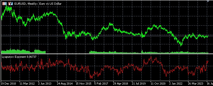
This indicator implements the calculation of the Lyapunov exponent for the analysis of financial time series. It allows assessing the degree of chaos in the market and the potential predictability of price movements.

Inputs:

input int    InpTimeLag = 1;       // Time lag
input int    InpEmbedDim = 2;      // Embedding dimension
input int    InpDataLength = 1000; // Data length for calculation

• InpTimeLag - time delay for phase space reconstruction.
• InpEmbedDim - embedding dimension for phase space reconstruction.
• InpDataLength - number of candles used to calculate the indicator.

There is one global variable:

double LyapunovBuffer[];

Initialization:

int OnInit()
{
   SetIndexBuffer(0, LyapunovBuffer, INDICATOR_DATA);
   IndicatorSetInteger(INDICATOR_DIGITS, 5);
   IndicatorSetString(INDICATOR_SHORTNAME, "Lyapunov Exponent");
   return(INIT_SUCCEEDED);
}

In the OnInit() function, we configure the indicator buffer, set the display precision to 5 decimal places, and set a short name for the indicator.

int OnCalculate(const int rates_total,
                const int prev_calculated,
                const datetime &time[],
                const double &open[],
                const double &high[],
                const double &low[],
                const double &close[],
                const long &tick_volume[],
                const long &volume[],
                const int &spread[])
{
   int start;
   if(prev_calculated == 0)
      start = InpDataLength;
   else
      start = prev_calculated - 1;
   
   for(int i = start; i < rates_total; i++)
   {
      LyapunovBuffer[i] = CalculateLyapunovExponent(close, i);
   }
   
   return(rates_total);
}

The OnCalculate() function is called on every tick and performs the calculation of the Lyapunov exponent for each candle starting from InpDataLength.

Lyapunov exponent calculation:

double CalculateLyapunovExponent(const double &price[], int index)
{
   if(index < InpDataLength)
      return 0;
   
   double sum = 0;
   int count = 0;
   
   for(int i = 0; i < InpDataLength - (InpEmbedDim - 1) * InpTimeLag; i++)
   {
      int nearestNeighbor = FindNearestNeighbor(price, index - InpDataLength + i, index);
      if(nearestNeighbor != -1)
      {
         double initialDistance = MathAbs(price[index - InpDataLength + i] - price[nearestNeighbor]);
         double finalDistance = MathAbs(price[index - InpDataLength + i + InpTimeLag] - price[nearestNeighbor + InpTimeLag]);
         
         if(initialDistance > 0 && finalDistance > 0)
         {
            sum += MathLog(finalDistance / initialDistance);
            count++;
         }
      }
   }
   
   if(count > 0)
      return sum / (count * InpTimeLag);
   else
      return 0;
}

The CalculateLyapunovExponent() function implements the algorithm for calculating the local Lyapunov exponent. It uses the nearest neighbor method to estimate the divergence of trajectories in the reconstructed phase space.

Searching for the nearest neighbor:

int FindNearestNeighbor(const double &price[], int startIndex, int endIndex)
{
   double minDistance = DBL_MAX;
   int nearestIndex = -1;
   
   for(int i = startIndex; i < endIndex - (InpEmbedDim - 1) * InpTimeLag; i++)
   {
      if(MathAbs(i - startIndex) > InpTimeLag)
      {
         double distance = 0;
         for(int j = 0; j < InpEmbedDim; j++)
         {
            distance += MathPow(price[startIndex + j * InpTimeLag] - price[i + j * InpTimeLag], 2);
         }
         distance = MathSqrt(distance);
         
         if(distance < minDistance)
         {
            minDistance = distance;
            nearestIndex = i;
         }
      }
   }
   
   return nearestIndex;
}

The FindNearestNeighbor() function finds the nearest point in the reconstructed phase space using Euclidean distance.

Interpretation of results

• Positive values of the indicator show the presence of chaotic market behavior.
• Negative values indicate more stable and potentially predictable price dynamics.
• The higher the absolute value of the indicator, the more pronounced the corresponding characteristic (chaotic or stable).

Statistical analysis of trend reversals and continuations using the Lyapunov exponent

I have developed a specialized script in the MQL5 language for an in-depth study of the relationship between the Lyapunov exponent and the dynamics of financial markets. This tool allows for detailed statistical analysis of trend reversals and continuations in the context of Lyapunov exponent values, providing traders and analysts with valuable insights into market behavior.

The script works with historical data of the selected financial instrument, analyzing a specified number of bars. For each bar, the local Lyapunov exponent is calculated using the phase space reconstruction and nearest neighbor search method. This approach allows us to assess the degree of chaos in the system at each specific point in time.

Simultaneously, the script analyzes price dynamics, identifying reversals and trend continuations. A reversal is defined as a situation where the current closing price is higher than the previous one, and the next one is lower than the current one (or vice versa). All other cases are considered as a continuation of the trend.

The key feature of the script is its ability to compare the moments of trend reversals and continuations with the values of the Lyapunov exponent. This allows us to identify statistical patterns between the chaotic behavior of the market and its price dynamics. The script calculates the number of trend reversals and continuations that occur with positive and negative values of the Lyapunov exponent.

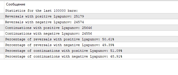
Upon completion of the analysis, the script displays detailed statistics, including absolute values and percentages of trend reversals and continuations for positive and negative values of the Lyapunov exponent. This information allows traders to assess how often trend reversals coincide with periods of increased market volatility, and conversely, how often trend continuations correspond to more stable periods.

Interpretation of statistical analysis results

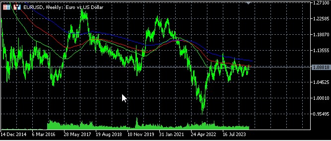
The obtained results of statistical analysis of trend reversals and continuations using the Lyapunov exponent provide interesting data on the dynamics of the EURUSD market on the hourly timeframe.

First of all, attention is drawn to the almost equal distribution of events between positive and negative values of the Lyapunov exponent. Both reversals and trend continuations are observed in approximately half of the cases with positive and negative Lyapunov exponents. This may indicate that the EURUSD market on H1 shows a balance between periods of relative stability and chaos.

Positive Lyapunov exponent values, which are typically associated with more chaotic, unpredictable behavior, are observed in just over half of all cases (50.61% for reversals and 51.09% for continuations). This may indicate a slight predominance of periods of increased volatility or uncertainty in the market.

Negative values of the Lyapunov exponent, usually interpreted as a sign of more orderly, less chaotic behavior of the system, are observed in 49.39% of reversals and 48.91% of trend continuations. These periods may be characterized by more predictable price movement, following certain patterns.

Interestingly, the percentage of trend reversals and continuations is almost identical for both positive and negative Lyapunov values. The difference is less than 0.5% in both cases. This may indicate that the Lyapunov exponent itself is not a determining factor for predicting a reversal or continuation of a trend.

This even distribution of events between positive and negative Lyapunov values may indicate the complex nature of the EURUSD market, where periods of stability and chaos alternate with approximately equal frequency. 

Conclusion

Chaos theory provides an innovative approach to analyzing financial markets, allowing for a deeper understanding of their complex and non-linear nature. In this article, we looked at the key concepts of chaos theory (attractors, fractals, and the butterfly effect) and their application to financial time series. Particular attention was paid to the Lyapunov exponent as a tool for assessing the degree of chaos in market dynamics.