
Neural Networks in Trading: Piecewise Linear Representation of Time Series

Introduction
Most often, when we talk about the presentation of a time series, we are presented with data that is a sequence of points recorded in chronological order. However, as the volume of initial information increases, the complexity of its analysis also increases, which reduces the efficiency of using the available information. This is especially important when working in financial markets, where extra time spent to analyze information and make decisions can lead to increased risks of lost profits, and sometimes even losses. This is where a special role is given to the advantages of reducing the dimensionality of data in order to increase the efficiency and effectiveness of their intellectual analysis. One approach to reducing the dimensionality of data is piecewise linear representation of time series.
Piecewise linear representation of time series is a method of approximating a time series using linear functions over small intervals. In this article, we will discuss the algorithm of Bidirectional Piecewise Linear Representation of time series (BPLR), which was presented in the paper "Bidirectional piecewise linear representation of time series with application to collective anomaly detection". This method was proposed to solve problems related to finding anomalies in time series.
Time series anomaly detection is a major subfield of time series data mining. Its purpose is to identify unexpected behavior throughout the data set. Since anomalies are often caused by different mechanisms, there are no specific criteria for their detection. In practice, data that exhibits expected behavior tends to attract more attention, while anomalous data is often perceived as noise which is usually ignored or eliminated. However, anomalies can contain useful information and thus detection of such anomalies can be important. Accurate anomaly detection can help mitigate unnecessary adverse impacts in various fields such as environment, industry, finance and others.
Anomalies in time series can be divided into the following three categories:
- Point anomalies: a data point is considered to be anomalous relative to other data points. These anomalies are often caused by measurement errors, sensor failures, data entry errors, or other exceptional events;
- Contextual anomalies: a data point is considered anomalous in a certain context, but not otherwise;
- Collective anomalies: a subsequence of a time series that exhibits anomalous behavior. This is quite a difficult task because such anomalies cannot be considered anomalous when analyzed individually. Instead, it is the collective behavior of the group that is anomalous.
Collective anomalies can provide valuable information about the system or process being analyzed, as they may indicate a group-level problem that needs to be addressed. Thus, detecting collective anomalies can be an important task in many fields such as cybersecurity, finance, and healthcare. The authors of the BPLR method focused in their work on identifying collective anomalies.
The high dimensionality of time series data requires significant computational resources when using the raw data for anomaly detection. However, to improve the performance of anomaly detection, a typical approach involves two phases: first performing dimensionality reduction and then using a distance measure to perform the task in the transformed representation subspace. Therefore, the authors of the method propose a new Bidirectional Piecewise Linear Representation (BPLR) algorithm. This method can transform the input time series into a low-dimensional expression form that is suitable for efficient analysis.
The paper also proposes a new similarity measurement algorithm based on the idea of piecewise integration (PI). It performs efficient similarity measure computation with a relatively low computational overhead.
1. The Algorithm
Anomaly detection based on the proposed BPLR method consists of two stages:
- Representing time series
- Measuring similarity
Before moving on to the description of the BPLR algorithm, I would like to emphasize that the method was developed to solve anomaly detection problems. It is assumed that the analyzed time series has some cyclicity, the size of which can be obtained experimentally or from a priori knowledge. Therefore, the entire input time series is divided into non-overlapping subsequences, the size of which is equal to the expected cycle of the original data. By comparing the obtained subsequences, the authors of the method try to find anomalous areas. Next, we describe an algorithm for representing one subsequence, which is repeated for all elements of the analyzed time series.
To perform the task of representing a time series, we need to find multiple sets of segmentation points in each subsequence. We then need transform the input subsequence into a set of linear segments.
First, in order to find the most probable points for splitting the subsequence into separate segments, we identify all possible Trend Turning Points, TTP. The authors of the method identify 6 variants of trend turning points.
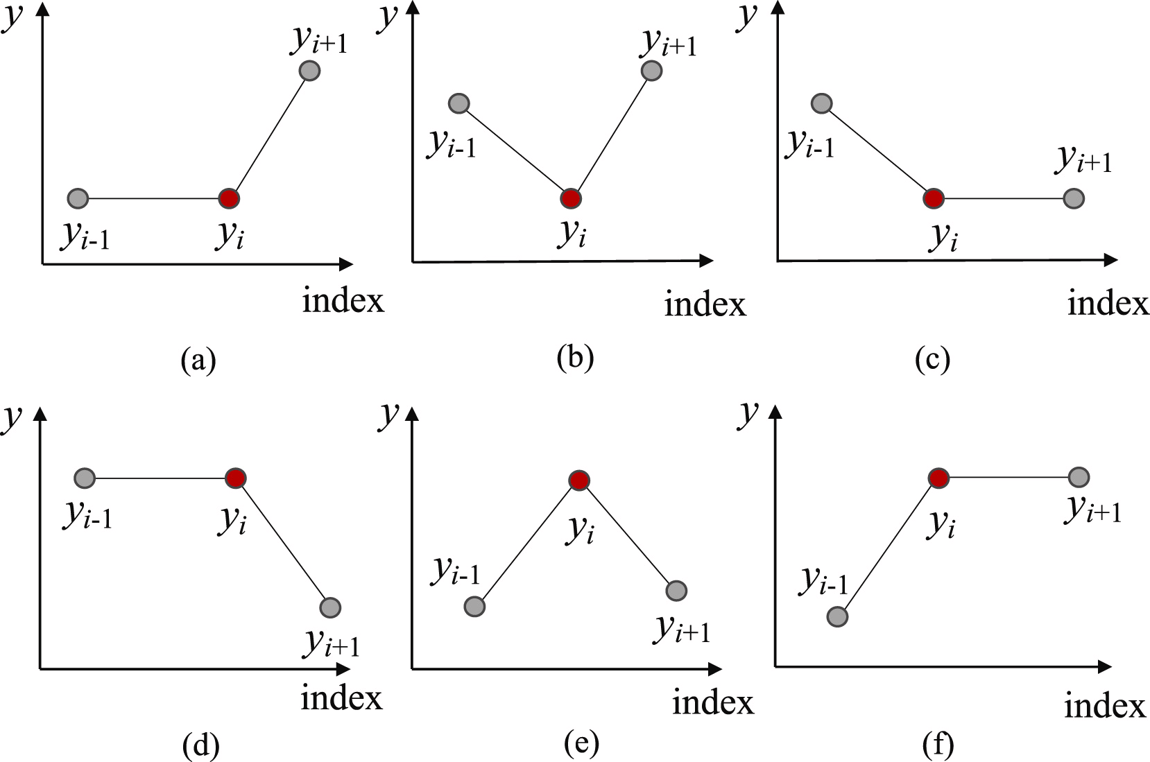
The first and last elements of the subsequence are automatically considered as trend turning points.
The next step is to determine the importance of each TTP found. As a measure of importance of TTP, the authors of the method propose to use the deviation from the mean value of the subsequence.

The TTPs are then sorted according to their importance. The segments are determined iteratively, starting with TTP1, with the highest importance in two directions: before and after TTP1. In this case, an additional hyperparameter δß is introduced to determine the quality of the segment. The hyperparameter defines the maximum allowable deviation of sequence points from the segment line.
To determine the starting point of the previous segment, we iterate over the elements of the input sequence in reverse order from the currently analyzed TTP1 while all elements between TTP1 and the candidate for the beginning of the segment are no further than δß. Once a point beyond this threshold is found, the search stops and the segment is saved. If previously found TTPs fall within the segment's coverage area, they are deleted.
Similarly we search for the end of the segment in the direction after TTP1. Since segments are searched in the directions before and after the extremum, method was called bidirectional.
After the end points of both segments have been determined, the operations are repeated with the extremum that is next in importance. The iterations are terminated when there are no unprocessed trend turning points left in the array.
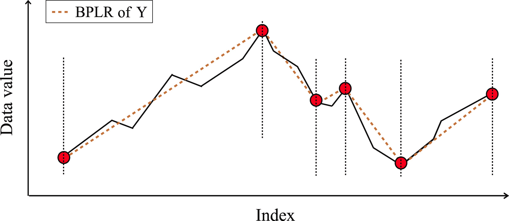
The similarity of two subsequences is determined based on the areas of the shapes formed by the segments of the analyzed sequences.
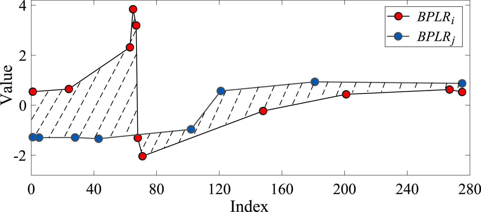
To solve the anomaly detection problem, the authors of the method create a distance matrix Mdist. Then, for each individual subsequence, they compute the total deviation from other subsequences of the analyzed time series Di. In practice Di represents the sum of the elements of the matrix Mdist in the ith row. A subsequence is considered anomalous if its total deviation differs from the relevant average value of the remaining subsequences.
In their paper, the authors of the BPLR method present the results of experiments on synthetic and real data, which show the effectiveness of the proposed solution.
2. Implementing in MQL5
We have discussed the theoretical representation of the BPLR method aimed at finding anomalous subsequences of time series. In the practical part of this article, we will implement our vision of the proposed approaches in MQL5. Please note that we will use the proposed solutions only partially.
Within the framework of our application area, we will not look for time series anomalies. Financial markets are very dynamic and multifaceted, so between any two disjoint subsequences, we will expectedly get significant deviations.
On the other hand, the alternative representation of the time series as a piecewise linear sequence can be quite useful. In the previous articles, we have already talked about the benefits of data segmentation. However, the question of determining the segment size still remained very relevant. For this purpose, we always used equal segment sizes. On the contrary, the piecewise linear representation method allows the use of dynamic segment sizes, depending on the analyzed input time series, which can assist in addressing the tasks of extracting features of time series of different scales. At the same time, the piecewise linear representation has a fixed size regardless of the segment size, which makes it convenient for analysis.
Another noteworthy part of the algorithm is the presentation of segments. The very name "piecewise linear representation" indicates the representation of a segment as a linear function:
![]()
As a result, we explicitly indicate the direction of the main trend in the time interval of the segment. Furthermore, the ability to compress data is an added bonus that helps reduce model complexity.
Of course, we will not divide the analyzed time series into subsequences. We will represent the entire set of initial data as a piecewise linear sequence. Our model, based on the analysis of the presented data, must draw conclusions and offer the "only correct" solution.
Let's start working with building a program on the OpenCL side.
2.1 Implementing on the OpenCL side
As you know, in order to optimize the model training and operating costs, we have moved the bulk of the computations to the context of OpenCL devices, which allowed us to organize computations in a multidimensional space. The current implementation is no exception in this regard.
To implement the segmentation of the analyzed time series, we create the PLR kernel.
__kernel void PLR(__global const float *inputs,
                  __global float *outputs,
                  __global int *isttp,
                  const int transpose,
                  const float min_step
                 )
  {
   const size_t i = get_global_id(0);
   const size_t lenth = get_global_size(0);
   const size_t v = get_global_id(1);
   const size_t variables = get_global_size(1);
In the parameters to the kernel, we plan to pass pointers to 3 data buffers:
- inputs
- outputs
- isttp – a service buffer for recording trend turning points
In addition, we will add 2 constants:
- transpose – flag indicating the need to transpose inputs and outputs
- min_step – the minimum deviation of subsequence elements to register a TTP
We will call the kernel in a 2-dimensional task space, in accordance with the number of elements in the analyzed sequence and the number of univariate sequences in the multidimensional time series. Accordingly, in the kernel body, we immediately identify the current flow in the task space, and then we define the constants for the offset in the input buffer.
//--- constants
   const int shift_in = ((bool)transpose ? (i * variables + v) : (v * lenth + i));
   const int step_in = ((bool)transpose ? variables : 1);
After a little preparatory work, we determine the presence of a TTP in the position of the analyzed element. The extreme points of the analyzed time series automatically receive the status of a trend turning point, since they are a priori the extreme points of the segment.
   float value = inputs[shift_in];
   bool bttp = false;
   if(i == 0 || i == lenth - 1)
      bttp = true;
In some cases, we first look for the closest deviation of the values of the analyzed series by the minimum required value before the current element of the sequence. At the same time, we save the minimum and maximum values in the iterated interval.
   else
     {
      float prev = value;
      int prev_pos = i;
      float max_v = value;
      float max_pos = i;
      float min_v = value;
      float min_pos = i;
      while(fmax(fabs(prev - max_v), fabs(prev - min_v)) < min_step && prev_pos > 0)
        {
         prev_pos--;
         prev = inputs[shift_in - (i - prev_pos) * step_in];
         if(prev >= max_v && (prev - min_v) < min_step)
           {
            max_v = prev;
            max_pos = prev_pos;
           }
         if(prev <= min_v && (max_v - prev) < min_step)
           {
            min_v = prev;
            min_pos = prev_pos;
           }
        }
Then, in a similar manner, we look for the next element with the minimum required deviation.
      //---
      float next = value;
      int next_pos = i;
      while(fmax(fabs(next - max_v), fabs(next - min_v)) < min_step && next_pos < (lenth - 1))
        {
         next_pos++;
         next = inputs[shift_in + (next_pos - i) * step_in];
         if(next > max_v && (next - min_v) < min_step)
           {
            max_v = next;
            max_pos = next_pos;
           }
         if(next < min_v && (max_v - next) < min_step)
           {
            min_v = next;
            min_pos = next_pos;
           }
        }
We check whether the current value is an extremum.
      if(
         (value >= prev && value > next) ||
         (value > prev && value == next) ||
         (value <= prev && value < next) ||
         (value < prev && value == next)
      )
         if(max_pos == i || min_pos == i)
            bttp = true;
     }
But here we should remember that when searching for elements with the minimum required deviation, we could collect a corridor of values from several elements of the sequence that form a certain extremum plateau. Therefore, an element receives a TTP flag only if it is an extremum in such a corridor.
Let's save the received flag and clear the output buffer. Here we also synchronize the local group threads.
//---
   isttp[shift_in] = (int)bttp;
   outputs[shift_in] = 0;
   barrier(CLK_LOCAL_MEM_FENCE);
We need to synchronize the threads in order to ensure that before further operations begin, all threads of the current univariate time series have recorded their flags of the presence of a TTP.
Further operations are performed only by threads in which a TTP is defined. The remaining threads do not meet the specified conditions and practically terminate.
Here we will first calculate the position of the current extremum. To do this, we count the number of positive flags for the current position of the element and save the position of the previous TTP within the input buffer in a local variable.
//--- calc position
   int pos = -1;
   int prev_in = 0;
   int prev_ttp = 0;
   if(bttp)
     {
      pos = 0;
      for(int p = 0; p < i; p++)
        {
         int current_in = ((bool)transpose ? (p * variables + v) : (v * lenth + p));
         if((bool)isttp[current_in])
           {
            pos++;
            prev_ttp = p;
            prev_in = current_in;
           }
        }
     }
After that, we will determine the parameters of the linear approximation of the current segment's trend.
//--- cacl tendency
   if(pos > 0 && pos < (lenth / 3))
     {
      float sum_x = 0;
      float sum_y = 0;
      float sum_xy = 0;
      float sum_xx = 0;
      int dist = i - prev_ttp;
      for(int p = 0; p < dist; p++)
        {
         float x = (float)(p);
         float y = inputs[prev_in + p * step_in];
         sum_x += x;
         sum_y += y;
         sum_xy += x * y;
         sum_xx += x * x;
        }
      float slope = (dist * sum_xy - sum_x * sum_y) / (dist > 1 ? (dist * sum_xx - sum_x * sum_x) : 1);
      float intercept = (sum_y - slope * sum_x) / dist;
Save the obtained results in the outputs buffer.
      int shift_out = ((bool)transpose ? ((pos - 1) * 3 * variables + v) : (v * lenth + (pos - 1) * 3));
      outputs[shift_out] = slope;
      outputs[shift_out + 1 * step_in] = intercept;
      outputs[shift_out + 2 * step_in] = ((float)dist) / lenth;
     }
Here we characterize each obtained segment by 3 parameters:
- slope — trend line slope;
- intercept — the shift of the trend line in the input subspace;
- dist — segment length.
Perhaps a few words should be said about the presentation of the segment duration (length). As you might have guessed, specifying the sequence length as an integer value is not the best result in this case. Because for the efficient operation of the model, a normalized data presentation format is preferable. Therefore, I decided to represent the segment duration as a fraction of the total size of the analyzed univariate time sequence. So, let's divide the number of elements in a segment by the number of elements in the entire sequence of the univariate time series. In order not to fall into the "trap" of integer operations, we will first convert the number of elements in the segment from int to the float type.
Additionally, we will create a separate branch of operations for the last segment. The point is that we do not know the number of segments that will be formed at any given point in time. Hypothetically, with significant fluctuations in the elements of the time series and the presence of trend turning points in each element of the time series, we can get 3 times more values instead of compression. Of course, such a case is unlikely, however, it's better to avoid an increase in the data volume. At the same time, we do not want to lose data.
Therefore, we proceed from a priori knowledge of the representation of time series in MQL5 and understanding the structure of the analyzed data: the latest data in time is at the beginning of our time series. So, we pay more attention to them. Data at the end of the analyzed window happened earlier in history and thus has less influence on subsequent events. Anyway, we do not exclude such an influence.
Therefore, to write the results, we use a data buffer size similar to the size of the input time series tensor. This allows us to write segments 3 times smaller than the sequence length (3 elements to write 1 segment). We expect that this volume is more than sufficient. However, we play it safe and if there are more segments, we merge the data of the last segments into 1 to avoid data loss.
   else
     {
      if(pos == (lenth / 3))
        {
         float sum_x = 0;
         float sum_y = 0;
         float sum_xy = 0;
         float sum_xx = 0;
         int dist = lenth - prev_ttp;
         for(int p = 0; p < dist; p++)
           {
            float x = (float)(p);
            float y = inputs[prev_in + p * step_in];
            sum_x += x;
            sum_y += y;
            sum_xy += x * y;
            sum_xx += x * x;
           }
         float slope = (dist * sum_xy - sum_x * sum_y) / (dist > 1 ? (dist * sum_xx - sum_x * sum_x) : 1);
         float intercept = (sum_y - slope * sum_x) / dist;
         int shift_out = ((bool)transpose ? ((pos - 1) * 3 * variables + v) : (v * lenth + (pos - 1) * 3));
         outputs[shift_out] = slope;
         outputs[shift_out + 1 * step_in] = intercept;
         outputs[shift_out + 2 * step_in] = ((float)dist) / lenth;
        }
     }
  }
In most cases, we expect to have fewer segments, and then the last elements of our result buffer will be filled with zero values.
It should be noted here that the algorithm presented above does not contain trainable parameters and can be used at the stage of preliminary preparation of the initial data. This does not imply the presence of a backpropagation process and error gradient distribution. However, in our work, we will implement this algorithm into our models. As a consequence, we will need to implement a backpropagation algorithm to propagate the error gradient from subsequent neural layers to the previous ones. Since there are no learnable parameters, there are no optimization algorithms for them.
Thus, as part of the implementation of the backpropagation algorithms, we will create the error gradient distribution kernel PLRGradient.
__kernel void PLRGradient(__global float *inputs_gr,
                          __global const float *outputs,
                          __global const float *outputs_gr,
                          const int transpose
                         )
  {
   const size_t i = get_global_id(0);
   const size_t lenth = get_global_size(0);
   const size_t v = get_global_id(1);
   const size_t variables = get_global_size(1);
In the kernel parameters we also pass pointers to 3 data buffers. However, this time we have 2 error gradient buffers (at the input and output levels) and a buffer of the current layer's feed-forward results. In addition, we will add the already familiar data transposition flag to the kernel parameters. This flag is used when determining offsets in data buffers.
We will call the kernel in the same 2-dimensional task space. The first dimension is limited by the size of the time series sequence, and the second one is limited by the number of univariate time series in the multimodal source data. In the kernel body, we first identify the current thread in the task space in all dimensions.
Next, we define constants for the offsets in the data buffers.
//--- constants
   const int shift_in = ((bool)transpose ? (i * variables + v) : (v * lenth + i));
   const int step_in = ((bool)transpose ? variables : 1);
   const int shift_out = ((bool)transpose ? v : (v * lenth));
   const int step_out = 3 * step_in;
But the preparatory work is not complete yet. Next, we need to find the segment that contains the analyzed input element. To find it, we run a loop and in the loop body we will the sizes of the segments, starting from the very first one. We will repeat the loop iterations until we find a segment that contains the desired input data element.
//--- calc position
   int pos = -1;
   int prev_in = 0;
   int dist = 0;
   do
     {
      pos++;
      prev_in += dist;
      dist = (int)fmax(outputs[shift_out + pos * step_out + 2 * step_in] * lenth, 1);
     }
   while(!(prev_in <= i && (prev_in + dist) > i));
After all loop iterations we get:
- pos — index of the segment containing the desired element of the input data
- prev_in — offset in the input data buffer to the first segment element
- dist — the number of elements in the segment
To calculate the first-order derivatives of feed-forward operations, we also need the sum of the positions of the segment elements and the sum of their square values.
//--- calc constants
   float sum_x = 0;
   float sum_xx = 0;
   for(int p = 0; p < dist; p++)
     {
      float x = (float)(p);
      sum_x += x;
      sum_xx += x * x;
     }
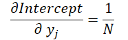
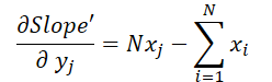
At this point, the preparatory work is complete and we can move on to computing the error gradient. First, we extract the error gradient for the slope and offset.
//--- get output gradient
   float grad_slope = outputs_gr[shift_out + pos * step_out];
   float grad_intercept = outputs_gr[shift_out + pos * step_out + step_in];
Now let's recall the formula we used in the feed-forward pass to compute the vertical shift of the trend line.
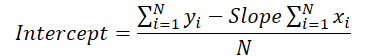
The line slope value is used to calculate the shift. Therefore, it is necessary to adjust the slope error gradient taking into account its influence on the shift adjustment. To do this, we find the derivative of the shift function with respect to the slope.
We multiply the obtained value by the shift error gradient and add the result to the slope error gradient.
//--- calc gradient
   grad_slope -= sum_x / dist * grad_intercept;
Now let's turn to the formula for determining the slope.
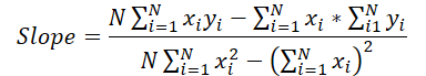
In this case, the denominator is a constant, and we can use it to adjust the slope error gradient.
grad_slope /= fmax(dist * sum_xx - sum_x * sum_x, 1);
And finally, let's look at the influence of the input data in both formulas.
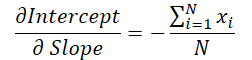
where 1 ≤ j ≤ N and
Using these formulas, let's determine the error gradient at the input data level.
   float grad = grad_intercept / dist;
   grad += (dist * (i - prev_in) - sum_x) * grad_slope;
   if(isnan(grad) || isinf(grad))
      grad = 0;
We save the result in the corresponding element of the input data gradient buffer.
//--- save result
   inputs_gr[shift_in] = grad;
  }
This concludes our work on the OpenCL context side. The full OpenCL code is provided in the attachment.
2.2 Implementing the new class
After completing operations on the OpenCL context side, we move on to working with the main program code. Here we will create a new class, CNeuronPLROCL, which will allow us to implement the above-described algorithm into our models in the form of a regular neural layer.
As in most similar cases, the new object will inherit its main functionality from our neural layer base class CNeuronBaseOCL. Below is the structure of the new class.
class CNeuronPLROCL  :  public CNeuronBaseOCL
  {
protected:
   bool              bTranspose;
   int               icIsTTP;
   int               iVariables;
   int               iCount;
   //---
   virtual bool      feedForward(CNeuronBaseOCL *NeuronOCL);
   //---
   virtual bool      calcInputGradients(CNeuronBaseOCL *prevLayer);
   virtual bool      updateInputWeights(CNeuronBaseOCL *NeuronOCL)  { return true; }

public:
                     CNeuronPLROCL(void)  : bTranspose(false) {};
                    ~CNeuronPLROCL(void) {};
   //---
   virtual bool      Init(uint numOutputs, uint myIndex, COpenCLMy *open_cl,
                          uint window_in, uint units_count, bool transpose,
                          ENUM_OPTIMIZATION optimization_type, uint batch);
   //---
   virtual int       Type(void)   const   {  return defNeuronPLROCL;   }
   //---
   virtual bool      Save(int const file_handle);
   virtual bool      Load(int const file_handle);
   virtual void      SetOpenCL(COpenCLMy *obj);
  };
The structure contains the redefinition of the standard set of methods with several additional variables. The purpose of the new variables can be understood from their names.
- bTranspose — flag indicating the need to transpose inputs and outputs
- iCount — the size of the sequence under analysis (history depth)
- iVariables — the number of analyzed parameters of a multimodal time series (univariate sequences)
Please note that although we have an auxiliary data buffer in the feed-forward pass kernel parameters, we do not create an additional buffer on the main program side. Here we only save a pointer to it in the local variable icIsTTP.
We do not have internal objects and thus we can leave the class constructor and destructor empty. The object is initialized in the Init method.
bool CNeuronPLROCL::Init(uint numOutputs, uint myIndex, COpenCLMy *open_cl,
                         uint window_in, uint units_count, bool transpose,
                         ENUM_OPTIMIZATION optimization_type, uint batch
                        )
  {
   if(!CNeuronBaseOCL::Init(numOutputs, myIndex, open_cl, window_in * units_count, optimization_type, batch))
      return false;
In the parameters, the method receives the main constants for defining the architecture of the created object. In the class body, we first call the method of the parent class with the same name, which already implements the necessary controls and initialization of inherited objects and variables.
Then we save the configuration parameters of the created object.
   iVariables = (int)window_in;
   iCount = (int)units_count;
   bTranspose = transpose;
At the end of the method, we create an auxiliary data buffer on the OpenCL context side.
   icIsTTP = OpenCL.AddBuffer(sizeof(int) * Neurons(), CL_MEM_READ_WRITE);
   if(icIsTTP < 0)
      return false;
//---
   return true;
  }
After initializing the object, we move on to constructing the feed-forward pass algorithm in the feedForward method. Here we just need to call the above-created feed-forward pass kernel PLR. However, it is necessary to create local groups to synchronize threads within individual univariate time series.
bool CNeuronPLROCL::feedForward(CNeuronBaseOCL *NeuronOCL)
  {
   if(!OpenCL || !NeuronOCL || !NeuronOCL.getOutput())
      return false;
//---
   uint global_work_offset[2] = {0};
   uint global_work_size[2] = {iCount, iVariables};
   uint local_work_size[2] = {iCount, 1};
To do this, we define a 2-dimensional global task space. For the first dimension, we indicate the size of the sequence being analyzed, and for the second dimension we indicate the number of univariate time series. We also define the size of the local group in a 2-dimensional task space. The size of the first dimension corresponds to the global value, and for the second dimension we specify 1. Thus, each local group gets its own univariate sequence.
Next, we just need to pass the necessary parameters to the kernel.
   ResetLastError();
   if(!OpenCL.SetArgumentBuffer(def_k_PLR, def_k_plr_inputs, NeuronOCL.getOutputIndex()))
     {
      printf("Error of set parameter kernel %s: %d; line %d", __FUNCTION__, GetLastError(), __LINE__);
      return false;
     }
   if(!OpenCL.SetArgumentBuffer(def_k_PLR, def_k_plr_outputs, getOutputIndex()))
     {
      printf("Error of set parameter kernel %s: %d; line %d", __FUNCTION__, GetLastError(), __LINE__);
      return false;
     }
   if(!OpenCL.SetArgumentBuffer(def_k_PLR, def_k_plt_isttp, icIsTTP))
     {
      printf("Error of set parameter kernel %s: %d; line %d", __FUNCTION__, GetLastError(), __LINE__);
      return false;
     }
   if(!OpenCL.SetArgument(def_k_PLR, def_k_plr_transpose, (int)bTranspose))
     {
      printf("Error of set parameter kernel %s: %d; line %d", __FUNCTION__, GetLastError(), __LINE__);
      return false;
     }
   if(!OpenCL.SetArgument(def_k_PLR, def_k_plr_step, (float)0.3))
     {
      printf("Error of set parameter kernel %s: %d; line %d", __FUNCTION__, GetLastError(), __LINE__);
      return false;
     }
And we put the kernel in the execution queue.
//---
   if(!OpenCL.Execute(def_k_PLR, 2, global_work_offset, global_work_size, local_work_size))
     {
      printf("Error of execution kernel %s: %d", __FUNCTION__, GetLastError());
      return false;
     }
//---
   return true;
  }
Do not forget to control operations at every stage. At the end of the method, we return the logical value of the method results to the caller.
The algorithm of the calcInputGradients error gradient distribution method is constructed in a similar way. But unlike the feed-forward pass method, here we do not create local groups, and each thread performs its operations independently. You can find the full code of all programs used in the article in the attachment below.
As mentioned above, the object we create does not contain learnable parameters. Therefore, the updateInputWeights parameter optimization method is redefined here only in order to preserve the general structure of objects and their compatibility during implementation. This method always returns true.
This concludes the description of the algorithms for implementing the methods of the new class. You can find the complete code of the class methods, including those not described in this article, in the attachment.
2.3 Model architecture
We have implemented one of the algorithms for piecewise linear representation of time series and can now add it to the architecture of our models.
To test the effectiveness of the proposed implementation, we have introduced a new class into the Environmental State Encoder model structure. I must say that we have considerably simplified the model architecture in order to evaluate the impact of the nominal decomposition of the time series on individual linear trends.
As before, we describe the architecture of the model in the CreateEncoderDescriptions method.
bool CreateEncoderDescriptions(CArrayObj *encoder)
  {
//---
   CLayerDescription *descr;
//---
   if(!encoder)
     {
      encoder = new CArrayObj();
      if(!encoder)
         return false;
     }
In parameters, the method receives a pointer to a dynamic array object for recording the architecture of the model. In the method body, we first check the relevance of the received pointer. After that, if necessary, we create a new instance of the dynamic array.
As usual, we feed the model with information about the state of the environment at a given depth of history without any data preprocessing.
//--- Encoder
   encoder.Clear();
//--- Input layer
   if(!(descr = new CLayerDescription()))
      return false;
   descr.type = defNeuronBaseOCL;
   int prev_count = descr.count = (HistoryBars * BarDescr);
   descr.activation = None;
   descr.optimization = ADAM;
   if(!encoder.Add(descr))
     {
      delete descr;
      return false;
     }
The piecewise linear representation algorithm works equally well with both normalized and raw data. But there are a few things to pay attention to.
First, in our implementation, we used the parameter of the minimum required deviation of the time series values to register a trend turning point. Needless to say, this requires careful selection of this hyperparameter for the analysis of each individual time series. The use of the algorithm to analyze multimodal time series, which have univariate sequences values lying in different distributions, significantly complicates this task. Furthermore, in most cases, this makes it impossible to use one hyperparameter for all analyzed univariate sequences.
Second, PLR results will be used in models whose efficiency is significantly higher when using normalized source data.
Of course, we can add normalization of PLR results before feeding them into the model, but even here the dynamic change in the number of segments complicates the task.
At the same time, normalization of input data before feeding it into the piecewise linear representation layer significantly simplifies all of the above points. By normalizing all univariate sequences to a single distribution, we can use one hyperparameter to analyze multimodal time series. Moreover, normalizing the distribution of the input data allows us to use average hyperparameters for completely different input sequences.
Having received normalized data at the input of the layer, we have normalized sequences at the output. Therefore, the next layer of our model is the batch normalization layer.
//--- layer 1
   if(!(descr = new CLayerDescription()))
      return false;
   descr.type = defNeuronBatchNormOCL;
   descr.count = prev_count;
   descr.batch = 1e4;
   descr.activation = None;
   descr.optimization = ADAM;
   if(!encoder.Add(descr))
     {
      delete descr;
      return false;
     }
Then, to work within univariate sequences, we transpose the input data.
//--- layer 2
   if(!(descr = new CLayerDescription()))
      return false;
   descr.type = defNeuronTransposeOCL;
   descr.count = HistoryBars;
   descr.window = BarDescr;
   if(!encoder.Add(descr))
     {
      delete descr;
      return false;
     }
Of course, in our implementation of the PLR algorithm, it could be more efficient to use the transposition parameter instead of using a data transposition layer. However, in this case, we use exactly the transposition due to the further construction of the model architecture.
Next, we will split the prepared data into linear segments.
//--- layer 3
   if(!(descr = new CLayerDescription()))
      return false;
   descr.type = defNeuronPLROCL;
   descr.count = HistoryBars;
   descr.window = BarDescr;
   descr.step = int(false);
   descr.activation = None;
   descr.optimization = ADAM;
   if(!encoder.Add(descr))
     {
      delete descr;
      return false;
     }
We use a 3-layer MLP for forecasting individual univariate sequences for a given planning horizon.
//--- layer 4
   if(!(descr = new CLayerDescription()))
      return false;
   descr.type = defNeuronConvOCL;
   descr.count = BarDescr;
   descr.window = HistoryBars;
   descr.step = HistoryBars;
   descr.window_out = LatentCount;
   descr.activation = LReLU;
   descr.optimization = ADAM;
   if(!encoder.Add(descr))
     {
      delete descr;
      return false;
     }
//--- layer 5
   if(!(descr = new CLayerDescription()))
      return false;
   descr.type = defNeuronConvOCL;
   descr.count = BarDescr;
   descr.window = LatentCount;
   descr.step = LatentCount;
   descr.window_out = LatentCount;
   descr.optimization = ADAM;
   descr.activation = SIGMOID;
   if(!encoder.Add(descr))
     {
      delete descr;
      return false;
     }
//--- layer 6
   if(!(descr = new CLayerDescription()))
      return false;
   descr.type = defNeuronConvOCL;
   descr.count = BarDescr;
   descr.window = LatentCount;
   descr.step = LatentCount;
   descr.window_out = NForecast;
   descr.optimization = ADAM;
   descr.activation = TANH;
   if(!encoder.Add(descr))
     {
      delete descr;
      return false;
     }
Note that we use convolutional layers with non-overlapping windows to organize conditionally independent prediction of individual univariate sequence values. I use the definition of "conditionally independent forecasting" because the same weighting matrices are used to construct the forecast trajectories of all univariate sequences.
We transpose the predicted values into a representation of the input data.
//--- layer 7
   if(!(descr = new CLayerDescription()))
      return false;
   descr.type = defNeuronTransposeOCL;
   descr.count = BarDescr;
   descr.window = NForecast;
   descr.activation = None;
   if(!encoder.Add(descr))
     {
      delete descr;
      return false;
     }
We add to them the statistical parameters of the distribution, eliminated during the normalization of the original data.
//--- layer 8
   if(!(descr = new CLayerDescription()))
      return false;
   descr.type = defNeuronRevInDenormOCL;
   descr.count = BarDescr*NForecast;
   descr.activation = None;
   descr.optimization = ADAM;
   descr.layers=1;
   if(!encoder.Add(descr))
     {
      delete descr;
      return false;
     }
At the output of the model, we use the developments of the FreDF method to coordinate individual steps of the predictive univariate sequences of the analyzed time series that we constructed.
//--- layer 9
   if(!(descr = new CLayerDescription()))
      return false;
   descr.type = defNeuronFreDFOCL;
   descr.window = BarDescr;
   descr.count =  NForecast;
   descr.step = int(true);
   descr.probability = 0.7f;
   descr.activation = None;
   descr.optimization = ADAM;
   if(!encoder.Add(descr))
     {
      delete descr;
      return false;
     }
//---
   return true;
  }
So, we have built an Environmental State Encoder model, which unites PLR and MLP for time series forecasting.
3. Testing
In the practical part of this article, we implemented an algorithm for the piecewise linear representation (PLR) of time series. The proposed algorithm does not contain learnable parameters. Instead, it involves transforming the analyzed time series into an alternative representation. We also presented a rather simplified time series forecasting model using the created layer CNeuronPLROCL. Now it's time to evaluate the effectiveness of these approaches.
To train the Environmental State Encoder model to predict subsequent indicators of the analyzed time series, we use the training dataset collected for the previous article.
We train models using real historical data of the EURUSD instrument with the H1 timeframe, collected for the entire year 2023. During the Environmental State Encoder model training, it works only with historical data of price movements and analyzed indicators. Therefore, we train the model until we get the desired result, without the need to update the training dataset.
Speaking about model training, I would like to note the stability of the process. The model learns quite quickly, without sharp jumps in forecast error.
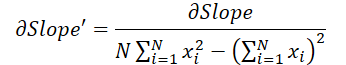
As a result, despite the relative simplicity of the model, we got a pretty good result. For example, below is a comparative chart of the target and forecast price movement.
The chart shows that the model was able to capture the main trends of the upcoming price movement. It is quite remarkable that with a 24-hour forecast horizon we have quite close values at the beginning and end of the forecast trajectory. Only the price movement momentum of the forecast trajectory is more extended in time.
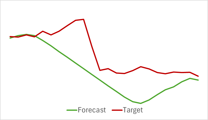
The forecast trajectories of the analyzed indicators also demonstrate good results. Below is a graph of the predicted RSI values.
The predicted values of the indicator are slightly higher than the actual values and have a smaller amplitude, but they are consistent in time and direction of the main impulses.
Please note that the presented forecasts of price movement and indicator readings refer to the same time period. If you compare the two presented graphs, you can see that the main momentum of the predicted and actual values of the indicators coincides in time with the main momentum of the actual price movement.
Conclusion
In this article, we have discussed methods for the alternative representation of time series in the form of piecewise linear segmentation. In the practical part of the article, we have implemented one of the variants of the proposed approaches. The results of the experiments conducted indicate the existing potential of the approaches considered.
References
Programs used in the article
| # | Name | Type | Description |
|---|---|---|---|
| 1 | Research.mq5 | EA | Example collection EA |
| 2 | ResearchRealORL.mq5 | EA | EA for collecting examples using the Real-ORL method |
| 3 | Study.mq5 | EA | Model training EA |
| 4 | StudyEncoder.mq5 | EA | Encoder training EA |
| 5 | Test.mq5 | EA | Model testing EA |
| 6 | Trajectory.mqh | Class library | System state description structure |
| 7 | NeuroNet.mqh | Class library | A library of classes for creating a neural network |
| 8 | NeuroNet.cl | Code Base | OpenCL program code library |
Translated from Russian by MetaQuotes Ltd.
Original article: https://www.mql5.com/ru/articles/15217
Warning: All rights to these materials are reserved by MetaQuotes Ltd. Copying or reprinting of these materials in whole or in part is prohibited.
This article was written by a user of the site and reflects their personal views. MetaQuotes Ltd is not responsible for the accuracy of the information presented, nor for any consequences resulting from the use of the solutions, strategies or recommendations described.

 MetaTrader 5 on macOS
- Free trading apps
- Over 8,000 signals for copying
- Economic news for exploring financial markets
You agree to website policy and terms of use