Quantization in machine learning (Part 1): Theory, sample code, analysis of implementation in CatBoost

Introduction

The article considers the theoretical application of quantization in the construction of tree models No complex mathematical equations are used. While writing the article, I discovered the absence of established unified terminology in the scientific works of different authors, so I will choose the terminology options that, in my opinion, best reflect the meaning. Besides, I will use the terms of my own in the matters left unattended by other researchers. This article will use terms and concepts I have previously described in the article "CatBoost machine learning algorithm from Yandex without learning Python or R". Therefore, I recommend that you familiarize yourself with it before reading the current article.

This article will not consider the possibility of applying quantization to trained neural networks in order to reduce their size, since I currently have no personal experience in this matter.

Here is what you can expect: 

• The first part of the article contains introductory theoretical material about quantization, and will be useful for understanding the goals and essence of the process.
• In the second part of the article, the uniform quantization method will be discussed using MQL5 code as an example.
• In the third part of the article, I will consider the implementation of the quantization process using CatBoost as an example.

 

1. Standard uses

So what is quantization and why is it used? Let's figure it out!

First, let's talk a little about the data. So, to create models (carry out training), we require data that is scrupulously collected in the table. The source of such data can be any information that can explain the target one (determined by the model, for example, a trading signal). Data sources are called differently - predictors, features, attributes or factors. The frequency of occurrence of a data line is determined by the occurrence of a comparable process observation of the phenomenon, about which information is being collected and which will be studied using machine learning. The totality of the data obtained is called a sample.

A sample can be representative - this is when the observations recorded in it describe the entire process of the phenomenon under study, or it can be non-representative when there is as much data as it was possible to collect, which allows only a partial description of the process of the phenomenon under study. As a rule, when we deal with financial markets, we are dealing with non-representative samples due to the fact that everything that could happen has not yet happened. For this reason, we do not know how the financial instrument will behave in case of new events (that have not occurred before). However, everyone knows the wisdom "history repeats itself". It is this observation that the algorithmic trader relies on in its research, hoping that among the new events there will be those that were similar to the previous ones, and their outcome will be similar with the identified probability.

According to their logical content (according to the measurement scale), the numerical indicators of predictors can be:

• Binary – confirm or refute the presence of a fixed attribute of the observed phenomenon;
• Quantitative (metric scale) - describes a phenomenon with some kind of measuring indicator, for example, it can be speed, coordinates of something, size, time elapsed since the beginning of an event and many other characteristics that can be measured, including derivatives from them.
• Categorical (nominal scale) - signals about different observable objects or phenomena included in one logical group, as a rule, expressed as an integer. For example, days of the week, direction of the price trend, serial number of the support or resistance level.
• Rank (ordinal scale) - characterize the degree of superiority or ordering of something. It is rarely allocated to a separate group, since it can be classified as other types of indicators depending on the context and logic. For example, this can include the order of actions, the result of an experiment in the form of an assessment of its outcome relative to other similar experiments.

So, the sample contains different predictors with their own numerical indicators, and these data, in their totality, describe the observed phenomenon, the characteristics or type of which is described in the target function (hereinafter referred to as the target function). The target function in the sample can be either a numerical indicator or a categorical one. Further in the text, I will consider categorical target function, and to a greater extent a binary one.

Wikipedia offers the following definition:

Quantization — in mathematics and digital signal processing, is the process of mapping input values from a large set (often a continuous set) to output values in a (countable) smaller set, often with a finite number of elements. The signal value can be rounded either to the nearest level, or to the lower or higher of the nearest levels, depending on the encoding method. This quantization is called scalar. There is also vector quantization — partitioning the space of possible values of a vector quantity into a finite number of regions and replacing these values with the identifier of one of these regions. 

 I like the shorter definition:

Data quantization is a method of compressing (encoding) observation information with an acceptable loss of accuracy in its measurement scale. Compression (coding) implies discreteness of objects, which implies their same type and homogeneity, or simply similarity. The similarity criterion may be different, depending on the chosen algorithm and the logic embedded in it.

Data quantization is used everywhere, especially in the conversion of an analog signal to a digital one, as well as in the subsequent compression of the digital signal. For example, the data received from the camera matrix can be recorded as a raw file, and then immediately (or later on a computer) compressed into jpg or another convenient data storage format.

Looking at the graphical representation of data, in the form of candles or bars in the MetaTrader 5 terminal, we already see the result of the work of quantizing ticks on the time scale we have chosen. Quantizing a continuous data stream over time is usually called sampling (or discretization).

Typically, sampling is the process of recording observation characteristics at a given frequency over time. However, if we assume that this is the frequency with which data is collected into a sample, then the definition should be adjusted to the following: "Sampling is the process of recording observation characteristics, the frequency of which is determined by a given function during its threshold activation". A function here means any algorithm that, according to its own inherent logic, gives a signal to receive data. For example, in MetaTrader 5 we see exactly this approach, because on non-trading days, instead of repeating the closing price as a process that lasts over time, there is simply no information on the chart, i.e. the sampling rate drops to zero.

A simple example of a quantization algorithm is the construction of a histogram. The algorithm for this method is quite simple:

• Find the maximum and minimum values of the indicator (in our case, the predictor).
• Calculate the difference between the maximum and minimum indicators.
• Divide the resulting delta in point 2 by an integer, for example, ten, or, depending on the number of observations (as recommended by Karl Pearson). Obtain the division step in the initial units of measurement, which will be the reading of the new measurement scale.
• Now we need to build our own scale with our own divisions. This is done simply by multiplying the step by the serial number of the reading.
• Next, each observation value is assigned to the range of a new measurement scale and the number of observations in each range is summed up separately.

The algorithm result is a histogram displayed in Figure 1.

 

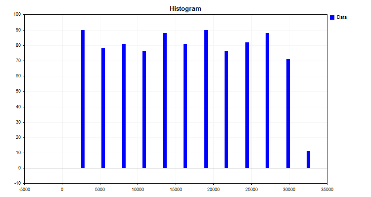
Figure 1

The histogram shows how the data is distributed according to the new measurement scale. Based on the appearance of the distribution, through the apparatus of descriptive statistics, one can assume the type of distribution density, which can be useful for choosing a finite quantization method. You can read about the distribution density in the following articles:

• Kernel density estimation of the unknown probability density function;
• Statistical Distributions in MQL5 - taking the best of R and making it faster;
• Statistical estimations.

So, what we got by building a histogram:

• Levels (cutoffs) or borders that divide the data into groups. A set of levels is called a quantum grid or dictionary - it is at these levels that the data encoding occurs, which ensures their grouping and compression. Borders can be installed according to different rules embedded in the quantization algorithm. Levels (cutoffs) form a new scale for measuring observational indicators. I am used to calling the range between two levels a "quantum segment", although other names are found in works of other authors — "interval", "range" or "quantization step";
• The belonging of each observation value (indicator) to a given group (histogram column). For quantization, this is the work of a compression algorithm, the essence of which is to transform the original data into compressed data at the moment of assigning the observation value to a certain range of the quantum grid. The result of compression can be various numerical transformation of the variable value. Two options are occurred most often: the first one is transformation, in which a variable is assigned a rank (index) according to the number of the range between the values of the cutoffs (borders), in which the number falls, and the second option is the assignment of a level scale value to the variable, for example, the numerical value of an observation falls in the range between 1.2 and 1.4, then the right value is assigned - 1.4. However, to use the second option, we need to set limits, beyond which the data will not go, while the first option allows you to work with any values outside the boundaries of the quantum table. For the second option, a good solution might be to force the addition of levels (borders/boundaries) at a considerable distance, which will allow errors in the form of spikes or missing data to be placed there.
• The ability to restore each number value with loss of accuracy (dequantization), which can be done in the following ways:
• - Along the center of the interval, which corresponds to the index of the number.
• - By the left or right level value (boundary/cutoff/border) of the interval, most often the right one. Considering that the boundaries in the quantization table are usually not defined for the first and last interval, then we can use the average range of intervals or the first and last values of the interval width to determine them.

Depending on the task and area of quantization application, one has to deal with different designations of variables and the style of writing equations, which makes it difficult to understand the essence of the algorithm, since the author describing them assumes knowledge from the specific area where the algorithm is applied. The essence of different algorithms comes down to different ways of constructing levels (cutoffs), so I propose to classify them according to a number of criteria.

Quantization with constant interval:

• Dividing into fixed intervals using a method similar to the Pearson histogram;
• Conversion to reduce the digit of a number.

Variable interval quantization:

• Accumulation of a fixed percentage of observations for each interval.
• Using a fixed value for the area under the curve of a theoretical or approximate distribution.
• Using a given function that changes the quantization step depending on the coefficient. These are often functions that extend the spacing toward the edge or toward the center.
• Using weighting coefficients that affect the interval, depending on the density of values.
• Iterative methods (including adaptive ones). Information about the data structure is used to configure the borders, and actions are taken to reduce the error.
• Other methods.

Quantization with an empirically determined interval:

• Number sequences;
• Knowledge about the nature of observation, allowing to group indicators that are similar in meaning;
• Manual marking.

Reducing the quantization error in the selected metric can be an iterative process, or it can be calculated once using a given equation. To evaluate the result, it is convenient to use the average percentage of error spread relative to the entire range of numbers that take the value of the predictor in the sample.

 

2. Implementing a quantization algorithm in MQL5

Previously, we looked at a simple example of how quantization works, but it lacks one of the steps that is often used in quantization, namely, re-partitioning the scale obtained after some calculations in order to find the average value of the interval, which is often called the centroid. The interval for quantization will be finally determined by half the distance between the boundaries of two nearby centroids.

Let's consider a step-by-step quantization of real numbers, such as double, which take up 8 bytes in memory, into the whole uchar data type, which takes up only 8 bits:

• 1. Finding the maximum and minimum in the input data:
• 1.1. Find the maximum and minimum values - Max and Min variable in the arr_In_Data array.
• 2. Calculate the window size between intervals:
• 2.1. Find the difference between the maximum and minimum and store it in the Delta variable.
• 2.2. Find the size of one window Delta/nQ, where nQ is the number of separators (borders), save the result in the Interval_Size variable.
• 3. Perform quantization and error calculation:
• 3.1. Shift the minimum value of the input data to zero arr_In_Data-Min.
• 3.2. Divide the result of point 3.1 by the number of Interval_Size intervals, which are one more than the number of separators.
• 3.3. Now we should apply the 'round' function, which rounds the number to the nearest integer, to the result obtained in 3.2. The result will be saved in the arr_Output_Q_Interval array.
• 3.4. Multiply the value from the arr_Output_Q_Interval array by Interval_Size and add the minimum. Now we have the converted (quantized) value of the number, which we will save in the arr_Output_Q_Data array.
• 3.5. Let's calculate the error as a cumulative total. To do this, we divide the difference in absolute value between the original value and the one obtained as a result of quantization by the range. Divide the resulting total by the number of elements in the arr_In_Data array.
• 4. Save the separators (borders) into the arr_Output_Q_Book array:
• 4.1. For the first interval, we make an amendment - add half the size of the interval (Interval_Size) to the minimum value (Min).
• 4.2. Subsequent intervals are calculated by adding the interval value to the value of the arr_Output_Q_Book array at the previous step.

Below is an example of a function code with the description of variables and arrays.

/+---------------------------------------------------------------------------------+
//|Quantization of transformation (encoding) type to a given integer bitness
//+---------------------------------------------------------------------------------+
double Q_Bit(
   double &arr_Input_Data[],//Quantization data array
   int &arr_Output_Q_Interval[],//Outgoing array with intervals containing data 
   double &arr_Output_Q_Data[],//Outgoing array with restored values of the original data 
   float &arr_Output_Q_Book[],//Outgoing array - "Book with boundaries" or "Quantization table"
   int N_Intervals=2,//Number of intervals the original data should be divided (quantized) into
   bool Use_Max_Min=false,//Use/do not use incoming maximum and minimum values
   double Min_arr=0.0,//Maximum value
   double Max_arr=100.0//Minimum value
)
{
   if(N_Intervals<2)return -1;//There may be at least two intervals, in this case, there is one separator
//---0. Initialize the variables and copy the arr_Input_Data array
   double arr_In_Data[];
   double Max=0.0;//Maximum
   double Min=0.0;//Minimum
   int Index_Max=0;//Maximum index in the array
   int Index_Min=0;//Minimum index in the array
   double Delta=0.0;//Difference between maximum and minimum
   int   nQ=0;//Number of separators (borders)
   double Interval_Size=0.0;//Interval size
   int Size_arr_In_Data=0;//arr_In_Data array size
   double Summ_Error=0.0;//To calculate error/data loss
   nQ=N_Intervals-1;//Number of separators
   Size_arr_In_Data=ArrayCopy(arr_In_Data,arr_Input_Data,0,0,WHOLE_ARRAY);
   ArrayResize(arr_Output_Q_Interval,Size_arr_In_Data);
   ArrayResize(arr_Output_Q_Data,Size_arr_In_Data);
   ArrayResize(arr_Output_Q_Book,nQ);

//---1. Finding the maximum and minimum in the input data
   if(Use_Max_Min==false)//If enforced array limits are not used
   {
      Index_Max=ArrayMaximum(arr_In_Data,0,WHOLE_ARRAY);
      Index_Min=ArrayMinimum(arr_In_Data,0,WHOLE_ARRAY);
      Max=arr_In_Data[Index_Max];
      Min=arr_In_Data[Index_Min];
   }

   else//Otherwise enforce the maximum and minimum 
   {
      Max=Max_arr;
      Min=Min_arr;
   }

//---2. Calculate the window size between intervals
   Delta=Max-Min;//Difference between maximum and minimum 
   Interval_Size=Delta/nQ;//Size of one window

//---3. Perform quantization and error calculation
   for(int i=0; i<Size_arr_In_Data; i++)
   {
      arr_Output_Q_Interval[i]=(int)round((arr_In_Data[i]-Min)/Interval_Size);
      arr_Output_Q_Data[i]=arr_Output_Q_Interval[i]*Interval_Size+Min;
      Summ_Error=Summ_Error+(MathAbs(arr_Output_Q_Data[i]-arr_In_Data[i]))/Delta;
   }
//---4. Save separators (borders) into the array
   for(int i=0; i<nQ; i++)
   {
      switch(i)
      {
      case 0:
         arr_Output_Q_Book[i]=float(Min+Interval_Size*0.5);
         break;
      default:
         arr_Output_Q_Book[i]=float(arr_Output_Q_Book[i-1]+Interval_Size);
         break;
      }
   }
   return Summ_Error=Summ_Error/(double)Size_arr_In_Data*100.0;
} 

Practical use of data quantization:

• Reducing the required memory for storing and processing data. This effect is achieved due to the fact that it is sufficient to store only the index of the quantum segment, in which the numerical value of the indicator number falls. In this case, it makes sense to change the data type from real double or float to integer types, such as int or even uchar.
• Accelerating calculations. Achieved by working with integers and reducing the set of numbers used, which reduces the number of cycles in the algorithms.
• Noise reduction. The quality of the source data may contain noise in the form of measurement errors, both primary - loss of data from the broker, and in the form of delays, rounding and measurement errors. Quantization averages the indicator in the range of the quantum segment, which smooths out such noise and does not allow the model to focus attention on it.
• Compensation for the lack of close observation values. Sometimes a predictor value is very rare due to a lack of observations and cannot be considered a spike. Quantization can give such observations a sufficient range of value dispersion to make the model usable on new data that was not in the sample.
• Fighting the curse of dimensionality. Reducing the number of possible combinations reduces the grid of possible coordinates of measurement spaces speeding up and improving training.

Two examples have showcased two main quantization strategies:

• Data approximation strategy.
• Data aggregation strategy.

The first type of strategy is most suitable for metric scales, which measure indicators that have distribution of characteristic values close to a continuous one. Theoretically, the more intervals that separate the range of values, the better, since the error in the scatter of the reconstructed value over the entire range of the number series will be smaller. This type is well suited for restoring mathematical functions.

The second type of strategy is aimed at grouping data. One can imagine that generalized categorical values of features are being created, and here the task of correctly estimating boundaries is much more difficult. In my experience, we need to ensure that at least 5% of observations from the sample fall into the interval.

It is worth noting that those features that are already categorical in meaning, without any conventions, should be quantized very carefully, combining only those that are truly similar. Moreover, similarity here implies the similarity of the sample when divided into subsamples.

Attached to the article is the script "Q_Trans", which serves as an example of the quantization process. The data for quantization is randomly generated. The script contains the following main functions:

• "Q_Bit" - quantization of conversion (encoding) type to a given integer bit depth
• "Book_to_cifra" - Decoder restores the approximate value of a number from the Quantization Table, an array with indices is required.
• "Book_to_cifra_v2" - Decoder restores the approximate value of a number from the Quantization Table, an array with indices is not required.
• "Q_Random" - Quantization with random boundaries.

The script contains the following settings:

• The number of intervals the original data should be divided (quantized) into;
• Initializing number for the random number generator;
• Save charts;
• Directory for saving charts;
• Chart width;
• Chart height;
• Font size.

 

Description of the script operation stages:

1. A sample will be generated randomly.

2. The chart of the trading instrument will display a histogram chart constructed as described earlier in the article (Figure 1), as well as the chart with the values of the generated predictor distributed in chronological order and divided by boundaries obtained after quantization (Figure 2). If "Save charts" is "true", the charts will be saved in the directory with custom terminal files "Files\Q_Trans\Grafics".

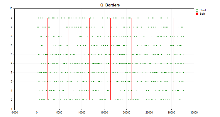   Figure 2.

3. The Q_Bit function is used to perform quantization and calculate the error in the form of an offset of the reconstructed value relative to the entire range of sample values.
4. The Book_to_cifra function is used to perform dequantization along the centroid and calculate the error in the form of an offset of the reconstructed value.
5. The Book_to_cifra function is used to perform dequantization along the right border and calculate the error in the form of an offset of the reconstructed value.
6. The Book_to_cifra_v2 function is used to perform dequantization along the centroid and calculate the error in the form of an offset of the reconstructed value.
7. Using the Q_Random function, 1000 attempts will be made to find the best intervals to split the predictor.
8. The Book_to_cifra function is used to perform dequantization along the centroid using a randomly obtained best grid and calculate the error in the form of an offset of the reconstructed value.

If we run the script with the default settings, then in the Experts terminal log, we will see the following information in the Message column

Average data recovery error size = 3.52% of full range when using 8 intervals
Average error size via quantum table for centroid conversion (Book_to_cifra) = 1145.62263
Average error size via quantum table for right boundary conversion (Book_to_cifra) = 2513.41952
Average error size via quantum table for centroid transformation (Book_to_cifra_v2) = 1145.62263
Average error size via quantum table for centroid transformation (Q_Random) = 1030.79216

The interesting thing is that the random method of selecting boundaries showed even better results than the one we considered earlier (based on uniform quantization).

 

3. Quantizations using CatBoost

CatBoost I previously wrote about in my article "CatBoost machine learning algorithm from Yandex without learning Python or R" uses quantization for data preprocessing, which can significantly speed up the operation of the gradient boosting algorithm. As before, I will use the console version of CatBoost, since it does not require the installation of additional software when performing work on the computer's central processor.

We will need the following settings:

1. Quantization (division) method – key "--feature-border-type":

• Median
• Uniform
• UniformAndQuantiles
• MaxLogSum
• MinEntropy
• GreedyLogSum

2. Number of separators from 1 to 65535 – key "--border-count"

3. Saving quantization tables to the specified file - key " --output-borders-file"

4. Loading quantization tables from the specified file – key " --input-borders-file"

 

If we do not specify the keys described above, then the following settings are used to build the models used in the article:

• For calculation on the CPU, the quantization method is "GreedyLogSum", the number of separators is "254";
• For GPU calculations, the quantization method is "GreedyLogSum", the number of separators is "128".

   

Let's have a look at how to register these keys:

Set up quantization by setting the "Uniform" method and the number of separators to 30, save the quantization table to the Quant_CB.csv file

catboost-1.0.6.exe fit --learn-set train.csv          --test-set test.csv --column-description Test_CB_Setup_0_000000000 --has-header --delimiter ; --train-dir ..\Rezultat --feature-border-type Uniform --border-count 30 --output-borders-file Quant_CB.csv 

Load the quantization table from the Quant_CB.csv file and train the model

catboost-1.0.6.exe fit --learn-set train.csv          --test-set test.csv --column-description Test_CB_Setup_0_000000000 --has-header --delimiter ; --train-dir ..\Rezultat --input-borders-file Quant_CB.csv

 You can find the section on the developer's instructions relating to quantization settings here.

 

Let's see how quantization methods differ when applied to specific data. Below are the graphs in the form of gif files. Each new frame is the next method. The number of separators is 16.

 

Figure 2 "Data graph for the categorical predictor"

 

Figure 3 "Data graph for the predictor with values shifted to the left area"

 

Figure 4 "Data graph for the predictor with values shifted to the right area"

 

Figure 5 "Data graph for the predictor with values placed in the central area"

 

Figure 6 "Data graph for the predictor with a uniform distribution of values"

 

If we look at the structure of the file with the quantization table (in our case, it will be Quant_CB.csv), we will see two columns and many rows. The first column stores the serial number of the predictor to be used when training the model, while the second column stores the separator (border/level). The number of rows corresponds to the cumulative sum of delimiters, and the number in the first column changes after all delimiters have been listed.

 

  

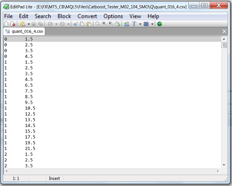
Table 1 "Contents of the saved CatBoost file with separators"

 

Conclusion

In this article, we got acquainted with the concept of quantization, analyzed obtaining quantized predictor values using MQL5 code as an example and examined the implementation of quantization in CatBoost.

If you detected terminology or factual errors in the article, feel free to contact me.

In the next article, we will figure out how to select quantum tables for a specific predictor and also conduct an experiment to assess the feasibility of this selection.

#	Application	Description
1	Q_Trans.mq5	Script containing an example of uniform quantization on a random sample.