MQL5 Wizard Techniques you should know (Part 74): Using Patterns of Ichimoku and the ADX-Wilder with Supervised Learning

Introduction

In the last article, we looked at the indicator pairing of Ichimoku and the ADX-Wilder as a complimentary S/R and trend tool pairing. As usual, we tested these in a wizard assembled Expert Advisor and looked at 10 different signal patterns. For this indicator pairing, most of them were able to forward walk profitably for 1-year, having done testing/ optimization on the previous year. However, there were 3 that did not do so satisfactorily and these were pattern-0, pattern-1, and pattern-5. We therefore follow up that article by examining if supervised learning can make a difference to their performance. Our approach in this is to reconstruct the signals of each of these patterns as a simple input vector into a neural network, essentially making the neural network an extra filter to the signal.

The Network

Our choice for a supervised learning model is a network that relies on a Spectral Mixture Kernel. This is defined by the following formula:

Where:

• τ \tau: Time difference between two points.
• Q: Number of spectral components.
• wi​: Weight of the i-th component (amplitude).
• li​: Length scale of the i-th component (controls decay).
• fi​: Frequency of the i-th component (oscillation rate).

We are using this spectral mixture kernel to define an entry layer to a simple neural network that has subsequent PyTorch-Linear layers after it. The kind of layer we are creating and using is a spectral mixture layer. We implement this layer and the regressor networks that follow it in python as indicated below:

class DeepSpectralMixtureRegressor(nn.Module):
    def __init__(self, input_dim=2, num_components=96):
        super().__init__()
        self.smk = DeepSpectralMixtureLayer(input_dim, num_components)
        feature_dim = input_dim * num_components  # 2 * 96 = 192

        self.head = nn.Sequential(
            nn.Linear(feature_dim, 1024),
            nn.ReLU(),
            nn.Linear(1024, 512),
            nn.ReLU(),
            nn.Linear(512, 256),
            nn.ReLU(),
            nn.Linear(256, 128),
            nn.ReLU(),
            nn.Linear(128, 1)  # <--- Removed sigmoid!
        )

    def forward(self, x):
        features = self.smk(x)
        output = self.head(features)
        return output

Some research does suggest using our special mixture kernel at the input serves to extract features from the input data, with the regression head of subsequent layers at the output being suitable in cases where the model is a regressor, as shown with our Sigmoid use. Our implemented choice of the spectral mixture kernel has the first layer performing periodic data modelling, while the regressor/head layers learn the frequencies, variances and weights of the network. Our implementation approach is best suited for regression tasks with oscillatory patterns in the input data. It also merges neural network flexibility with Gaussian Process Concepts.

Our network is named ‘DeepSpectralMixtureRegressor’. And we are engaging a modular Architecture that is two part. Feature-extraction and Regression. The first portion of feature-extraction is specifically handled by the ‘DeepSpectralMixtureLayer’ function, whose code we list below:

class DeepSpectralMixtureLayer(nn.Module):
    def __init__(self, input_dim, num_components):
        super().__init__()
        self.num_components = num_components
        hidden = 512  # Wider hidden layers

        # Go deeper with 4 layers
        def make_subnet():
            return nn.Sequential(
                nn.Linear(input_dim, hidden),
                nn.ReLU(),
                nn.Linear(hidden, hidden),
                nn.ReLU(),
                nn.Linear(hidden, hidden),
                nn.ReLU(),
                nn.Linear(hidden, num_components),
            )

        self.freq_net = make_subnet()
        self.var_net = nn.Sequential(*make_subnet(), nn.Softplus())
        self.weight_net = nn.Sequential(*make_subnet(), nn.Softplus())

    def forward(self, x):
        mu = self.freq_net(x)
        v = self.var_net(x)
        w = self.weight_net(x)

        expanded = x.unsqueeze(2)
        mu = mu.unsqueeze(1)
        v = v.unsqueeze(1)
        w = w.unsqueeze(1)

        x_cos = torch.cos(2 * np.pi * expanded * mu)
        x_exp = torch.exp(-v * expanded**2)
        features = w * x_exp * x_cos

        return features.flatten(start_dim=1)

Our function above learns frequencies, variances and weights through the use of neural networks. This ensures positivity, given that soft-plus activation is used for the variances and weights. The regression head maps the extracted features to a single output with sigmoid activation for bounded regression or binary classification. The case for this architecture is adaptability, with the model adapting to various data patterns. This can make it suitable for tasks like time series forecasting, especially if there are periodic components in the series. This ends up leveraging both the neural network and kernel-based approaches.

Wilson et al. (2013) note that spectral mixture kernels can be implemented in libraries like GPyTorch as covariance functions for use in the Gaussian Process of modelling periodic patterns if they represent spectral density as a mixture of components. Our approach thus adapts this concept into a neural network by parametrizing the kernel components of: frequency, variance and weights; through neural networks. This enables learned, data driven, feature extraction that can be especially relevant for problems such as time series forecasting where periodic/oscillatory patterns are present in the data. This was highlighted by Sebastian Callh in his blog post on spectral mixture kernels. Part of the inspiration in applying the kernel the way we are is also from this GPyTorch documentation. 

So, in a nutshell, instead of having a fixed kernel of parameters, our model uses neural networks to learn frequencies that are labelled mu, variances that we label v, and weights that we symbolize with w. This approach allows adaptation to various data patterns. The first feature extraction layer computes the features by using the formula ‘w * exp(-v * x^2) * cos(2πμx)’ that captures periodicity through cosine modulation with the smoothness of exponential decay. The modular design of having feature extraction as one layer via DeepSpectralMixtureLayer, and a regression head as a separate component enhances flexibility. The regression head for its part is a deep, fully connected network that maps features to a single output with the help of sigmoid activation. And this as already mentioned makes it suited for bounded regression or binary classification.

Let's take a deep dive into our code above to see how all that we are describing above gets implemented. Our code starts with standard imports for PyTorch and related libraries. These imports provide tools for tensor operations, neural network construction, optimization, data handling, and ONNX export of the trained model for inference in third party platforms. This is key for enabling building, training, and deploying of the model. This, as one would expect, is foundational not just for PyTorch-based development, but machine learning in general. For guidance, it is important to ensure compatibility between PyTorch and ONNX versions in order to have efficient data loading during training.

We then proceed to set our ‘DeepSpectralMixtureLayer’ initialization. This defines three neural networks, namely the frequency network, the variance network, and the weights network. Each of the networks maps the input to the number of component outputs, while using Soft plus activation that ensures the variances and weights remain positive as required by the kernel formulation. This is important because these networks separately parametrize the spectral mixture kernel to allow the data-driven feature extraction with Gaussian Process. The parameter ‘num_components’ controls the “feature-richness”. This parameter, num_components, can be tuned depending on the task complexity. Our use of soft plus activation avoids negative values that can lead to numerical instability.

We then set our forward pass function for the network. This function computes the spectral mixture features with the afore mentioned formula in the text above. It reshapes inputs and parameters so they can be broadcasted to the regression head. The application of cosine and exponential functions flattens the output for the regression layers. This core transformation mimics the spectral mixture kernel. The shape of the input ‘x’ should follow the format (batch_size, input_dim). Also, checks for numerical stability in ‘exp’ may require the clamping of the variance v. The parameter ‘num_components’ can be tuned to desired feature dimensionality.

With the feature extraction layer covered above, we can now turn to the regressor, the class called when defining the model. Its overarching goal is combining the spectral mixture layer described above with a fully connected head. This head maps kernel features to a single output in the 0-1 range via Sigmoid. The architecture head can be adjusted depending on task complexity by increasing layer sizes/number. Sigmoid can be removed for unbounded regression tasks. We finally also have a forward function, just like in the spectral layer function above. It passes input through the spectral mixture layer to extract features, then through the head for the final output. This forward function defines the complete forward pass, enabling end-to-end training and inference.

The input ‘x’ size should match the input-dim. An appropriate loss function such as BCE can be suitable, given the use of Sigmoid for activation. The parameter ‘num-components’ is very sensitive to the network’s performance, and its value sets the total of spectral components. Higher values increase expressiveness, however they risk overfitting. Starting  with a value of 64 and then tweaking it based on data complexity can be a sensible approach. Monitoring for overfitting when training can be crucial given the over expressive nature of the spectral mixture layer. Regularization and early stopping can help mitigate this.

Analysing learnt parameters of mu, v, and w can help understand periodic patterns as seen in these GPyTorch examples. When compared to typical Gaussian Process models, our approach lacks uncertainty estimates. Additional measures that quantify this could be supplemented. Finally, a forward pass can be computationally intense, especially when the parameter ‘num-components’ is very large or high dimension inputs are used. This is an additional consideration to keep in mind when fine-tuning and optimizing this model.

Indicator Implementations

From the signal patterns we tested in the last article, most of them were able to forward walk reasonably well, except for pattern-0, pattern-1, and pattern-5. To recap, we tested/optimized 10 signal patterns on the symbol GBP USD for the year 2023. We used the 30-minute timeframe unlike our typical 4-hour because signals of the Ichimoku are usually not that frequent on large time frames. Our forward walk as usual was on the year 2024. Even though 7 of the 10 patterns were able to forward walk profitably in 2025, our testing was only for 2 years, so further diligence and testing on extended periods of history prices is always recommended to the reader before what is presented here can be taken to a live trading environment.

With this background presented, let's look at how the indicator functions of Ichimoku and ADX Wilder are implemented in Python as well as their feature extracting functions for patterns 0,1,and 5.

Ichimoku in Python

We implement the Ichimoku function in Python as follows:

def Ichimoku(df, tenkan_period: int = 9, kijun_period: int = 26, senkou_span_b_period: int = 52, displacement: int = 26) -> pd.DataFrame:
    """
    Calculate Ichimoku Kinko Hyo components and append them to the input DataFrame.

    The components are:
        - Tenkan-sen (Conversion Line)
        - Kijun-sen (Base Line)
        - Senkou Span A (Leading Span A)
        - Senkou Span B (Leading Span B)
        - Chikou Span (Lagging Span)

    Args:
        df (pd.DataFrame): DataFrame with 'high', 'low', and 'close' columns.
        tenkan_period (int): Lookback period for Tenkan-sen (default 9).
        kijun_period (int): Lookback period for Kijun-sen (default 26).
        senkou_span_b_period (int): Lookback period for Senkou Span B (default 52).
        displacement (int): Forward displacement of Senkou spans and backward shift of Chikou span (default 26).
        
    Returns:
        pd.DataFrame: Input DataFrame with added Ichimoku columns.
    """
    # Input validation
    required_cols = {'high', 'low', 'close'}
    if not required_cols.issubset(df.columns):
        raise ValueError("DataFrame must contain 'high', 'low', and 'close' columns")
    if not all(p > 0 for p in [tenkan_period, kijun_period, senkou_span_b_period, displacement]):
        raise ValueError("All period values must be positive integers")

    result_df = df.copy()

    # Tenkan-sen (Conversion Line)
    high_tenkan = result_df['high'].rolling(window=tenkan_period).max()
    low_tenkan = result_df['low'].rolling(window=tenkan_period).min()
    result_df['Tenkan_sen'] = (high_tenkan + low_tenkan) / 2

    # Kijun-sen (Base Line)
    high_kijun = result_df['high'].rolling(window=kijun_period).max()
    low_kijun = result_df['low'].rolling(window=kijun_period).min()
    result_df['Kijun_sen'] = (high_kijun + low_kijun) / 2

    # Senkou Span A (Leading Span A)
    result_df['Senkou_Span_A'] = ((result_df['Tenkan_sen'] + result_df['Kijun_sen']) / 2).shift(displacement)

    # Senkou Span B (Leading Span B)
    high_span_b = result_df['high'].rolling(window=senkou_span_b_period).max()
    low_span_b = result_df['low'].rolling(window=senkou_span_b_period).min()
    result_df['Senkou_Span_B'] = ((high_span_b + low_span_b) / 2).shift(displacement)

    # Chikou Span (Lagging Span)
    result_df['Chikou_Span'] = result_df['close'].shift(-displacement)

    return result_df

Our coded function above computes the indicator components and appends them to the input data frame with default periods of 9 for Tenkan-sen, 26 for Kijun-sen, 26 for displacement and 52 for Senkou span B. The opening line of our code aims at validating our input. This ensures the data frame has necessary price columns and that period parameters are positive in order to prevent calculation errors. This step is critical for data integrity and avoiding runtime errors. Our indicator function needs to run on valid runtime data. It is always best practice to validate inputs before processing, to handle missing data or invalid parameters gracefully.

With the validation done, we proceed to calculate the Tenkan-sen. Our code computes the average of the highest high and lowest low over the past ‘tenkan-period’. Typically, we use a period of 9 and this acts as a short-term trend indicator. This buffer helps in signalling potential reversals when crossing Kijun-sen and this can be resourceful in making short-term trade decisions since it reflects recent price action. Adjustments can be made to the ‘Tenkan-period’ in order to achieve a desired sensitivity to short term price action. Shorter periods will have more sensitivity with longer periods being less so.

We then calculate the Kijun-sen buffer next. Similar to Tenkan-sen It's computed over a longer period, usually 26. This provides a medium-term trend indicator. Kijun-sen is important because it confirms trend direction and acts as a support/resistance. This tends to add a slightly more stable view of the markets when compared to the Tenkan-sen. It is useful in medium-term analysis, and in fact crossovers with the Tenkan-sen can serve as trading signals.

We then calculate the Senkou span A. This is simply the average of Tenkan-sen and Kijun-sen; shifted forward by the displacement period. This displacement is typically 26. This buffer forms one boundary of the Kumo cloud. It is crucial since it shows future support/resistance and this gives a forward-looking view on trend analysis as argued here. It is important to monitor the cloud’s relative position to price, with price above it pointing to a bullish outlook, while when below it would be bearish.

The Senkou span B calculation follows next, and here we are simply averaging the highest high and lowest low over a period that is usually 52, and shifted forward, forming the second boundary of the Kumo cloud. The Senkou B provides a longer-term view of support/resistance and enhances trend identification, particularly in larger time frames. For guidance, the cloud thickness, the distance between Senkou A and B, can be a proxy for volatility. Thus, thicker clouds can suggest stronger support/resistance.

Finally, we calculate the last buffer, the Chikou span. This buffer is simply the closing price shifted backward by the displacement period, typically 26, in order to compare current prices with past prices. It thus serves as a trend confirmation of whether current prices are above or below past prices, which is useful in confirming or validating a trend. The primary purpose of the Chikou therefore is confirmation, and this often requires sufficient history data to be present, given the use of displacements and long averaging periods.

ADX-Wilder in Python

With the Ichimoku defined in Python, we now turn to the ADX Wilder. This function computes the ADX by using Wilder’s method. Like with the Ichimoku, we append the input price data frame with additional buffers of ADX,  +DI, and -DI. This indicator uses a default period of 14, that could be adjusted for alignment with the Ichimoku or for attaining more price sensitivity; we use this 14 default nonetheless. We implement this in Python as follows:

def ADX_Wilder(df, period: int = 14) -> pd.DataFrame:
    """
    Calculate the Average Directional Index (ADX) using Wilder's method and 
    append the ADX, +DI, and -DI columns to the input DataFrame.

    ADX measures trend strength, while +DI and -DI measure trend direction.
    
    Args:
        df (pd.DataFrame): DataFrame with 'high', 'low', and 'close' columns.
        period (int): The lookback period to use. Default is 14.
        
    Returns:
        pd.DataFrame: Input DataFrame with 'ADX', '+DI', and '-DI' columns.
    """
    if not all(col in df.columns for col in ['high', 'low', 'close']):
        raise ValueError("DataFrame must contain 'high', 'low', and 'close' columns")
    if period <= 0:
        raise ValueError("Period must be a positive integer")

    result_df = df.copy()

    # Calculate directional movements
    up_move = result_df['high'].diff()
    down_move = result_df['low'].diff()

    plus_dm = np.where((up_move > down_move) & (up_move > 0), up_move, 0)
    minus_dm = np.where((down_move > up_move) & (down_move > 0), down_move, 0)

    # Calculate True Range (TR)
    high_low = result_df['high'] - result_df['low']
    high_close = np.abs(result_df['high'] - result_df['close'].shift(1))
    low_close = np.abs(result_df['low'] - result_df['close'].shift(1))
    tr = np.maximum(high_low, np.maximum(high_close, low_close))

    # Apply Wilder's smoothing
    atr = pd.Series(tr).rolling(window=period).mean()
    plus_di = 100 * pd.Series(plus_dm).rolling(window=period).sum() / atr
    minus_di = 100 * pd.Series(minus_dm).rolling(window=period).sum() / atr
    dx = 100 * np.abs(plus_di - minus_di) / (plus_di + minus_di)
    adx = dx.rolling(window=period).mean()

    result_df['+DI'] = plus_di
    result_df['-DI'] = minus_di
    result_df['ADX'] = adx

    return result_df

Off the bat, the first thing we do is validate the function's input. This as always ensures the necessary price columns are present and that the indicator period is also valid, in order to avoid calculation errors. All important for data integrity and operation on valid data. Also, cases of missing data should be handled appropriately. After validation, what we handle next are the directional movement calculations. These are the differences in highs and lows that determine the plus DM and the minus DM movements. They mark the strength of upward and downward trends, information that is key in trend direction sizing/analysis. It is important to ensure sufficient historical data in order to compute accurate directional differences. The data should also be monitored for gaps.

We then proceed to compute the true ranges. These are worked out as the greatest of the current high minus low, or high minus previous close, or low minus previous close. Absolute values from these differences are adopted for consistency. This range normalizes directional movements by making them comparable across different assets, as per ADX calculation requirements. It is essential to ensure no missing data in input price data frame to avoid errors from ‘NaN’ in the calculations.

We then proceed to calculate the smoother true range using a rolling mean. We also smooth the plus DM and minus DM buffers, normalizing the positive and negative directional indicators such that they are scaled to 100 for a percentage representation. The directional index, DX, a metric of trend strength, will thus be the absolute difference between plus DM and minus DM and normalized by their sum. Finally, the main indicator buffer, ADX, will be a smoothing of the DX over the indicator period, which in our case is 14. This final output then serves as the measure of a prevalent trend’s strength.

To recap from the last article, ADX provides trend strength values in the 0 to 100 range, with anything above 25 often taken to signify a strong trend. On the other hand, values below 20 are taken as a sign of weak or fledgling trends. The plus directional index and minus directional index quantify the strengths of bullish and bearish trends, respectively, with the difference between the two, potentially serving as an entry trade signal. The used period of 14 can also be adjusted to the required sensitivity, with smaller values leading to earlier signal and fractal point detection, while longer periods would be less volatile.

In applying the spectral mixture kernel via a regressive network as we defined after the introduction, we take our inputs from these two indicators in the form of a simple 2-dim vector. In some past articles, we have considered and explored the option of increasing the size of the input vector to our supervised learning networks by decomposing the various signals of each pattern into a boolean value, 0 or 1. This provided better results in training/optimization that failed to materialize on forward walking. So, presently the signals and patterns of each indicator are what we combine into a single boolean value, not its parts. The 2-dim has each dimension combining signals from 2 indicators. The first dim is solely concerned with confirming a bullish signal, while the second for a bearish signal.

Feature-0

We are applying the 3 laggard or poor performing features to our network of feature-0, feature-1, and feature-5. We implement feature-0 in Python as follows;

def feature_0(df):
    """
    """
    feature = np.zeros((len(df), 2))
    
    feature[:, 0] = ((df['close'].shift(1) < df['Senkou_Span_A'].shift(1)) &
                     (df['close'] > df['Senkou_Span_A']) &
                     (df['ADX'] >= 25.0)).astype(int)
    
    feature[:, 1] = ((df['close'].shift(1) > df['Senkou_Span_A'].shift(1)) &
                     (df['close'] < df['Senkou_Span_A']) &
                     (df['ADX'] >= 25.0)).astype(int)
    
    feature[0, :] = 0
    feature[1, :] = 0
    
    return feature

Our function starts by creating a blank NumPy array. This feature array that is sized to match the input data frame in rows, however it is assigned 2 columns. This provides a clean slate for generating signals and ensures no residue values affect the output. We then assign the value for the first column of this data frame, which is a check for the bullish signal. As per conditions we outlined in the last article, we get a 1 assignment to each row in this column of the NumPy array when the previous close is below Senkou span A, the current close is above the current Senkou span A, and ADX is at least 25. Detecting a bullish crossover where the price moves above Senkou span A often suggests an uptrend. The ADX being at least 25 ensures the signal occurs during a strong trend to reduce false positives of weak trending markets.

This assignment, using NumPy arrays, means the assignments are performed across multiple rows, concurrently. One of the chief reasons why developing and training models in Python is so clutch. We then assign the value for the bearish column, across all the array rows. Here, we set the column value, at each respective row, to 1 if the previous close is above the prior Senkou span A, the current close is below the current Senkou span A, and the ADX main buffer is at least 25. It spots the bearish crossover, which marks a sign of a potential downtrend. The ADX filter ensures the trend strength supports the signal.

Once we assign the bullish and bearish values, we then force the first two rows of our feature array to be zero, since they have no values and therefore a NaN. We were able to train our network on just this pattern, exported it as ‘74_0.onnx’ and imported it into a custom signal class of an MQL5 Expert Advisor. In the last article, this particular pattern failed to meaningfully forward walk, however when we test it now with the network serving as an extra filter to the indicator input signals, we get the following report;

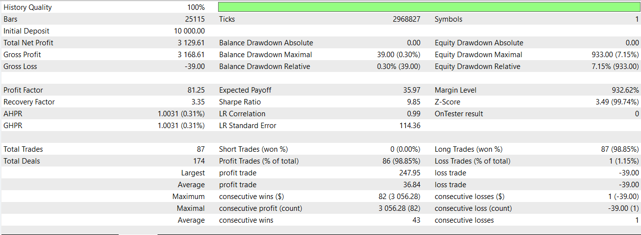
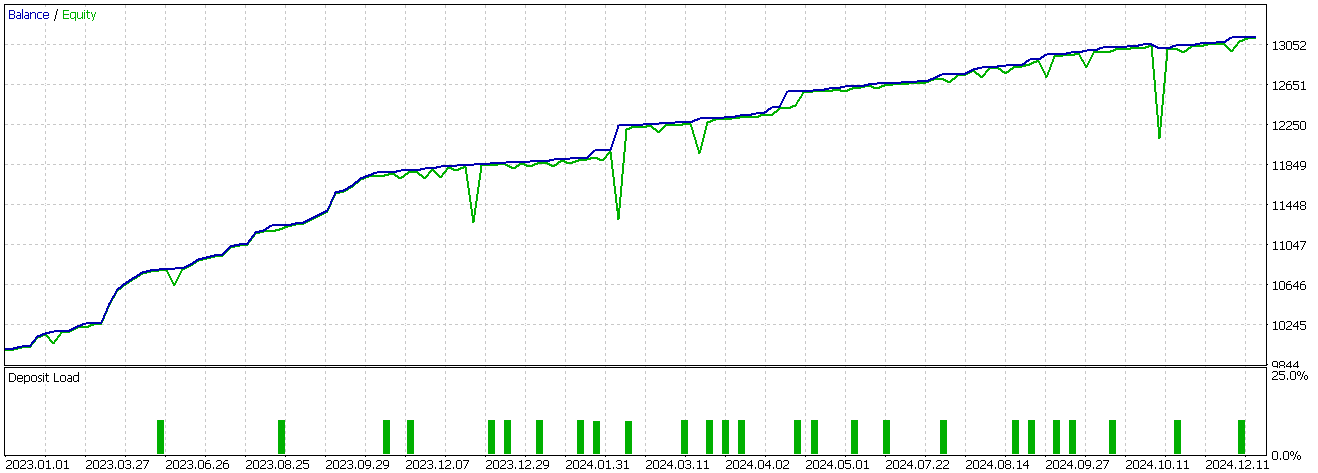
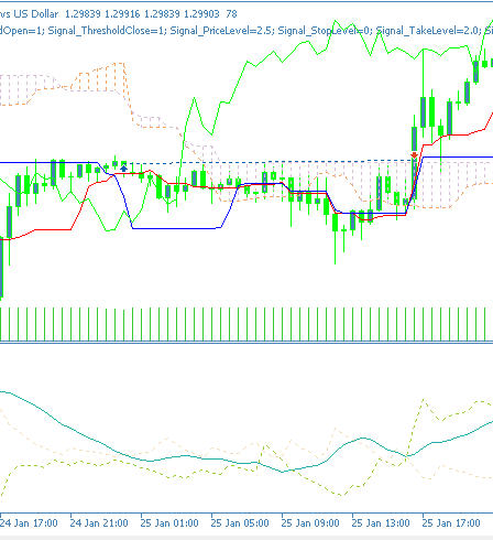
There appears to be a turn in fortunes however this is with only long positions placed and as always our testing is very limited in data scope and is thus only exploratory. A buy chart signal for feature-0, looks as follows on a chart;

Feature-1

Another feature/pattern that had dismal performance in the last article was feature-1. We implement this in Python as follows:

def feature_1(df):
    """

    """
    feature = np.zeros((len(df), 2))
    
    feature[:, 0] = ((df['Tenkan_sen'].shift(1) < df['Kijun_sen'].shift(1)) &
                     (df['Tenkan_sen'] > df['Kijun_sen']) &
                     (df['ADX'] >= 20.0)).astype(int)
    
    feature[:, 1] = ((df['Tenkan_sen'].shift(1) > df['Kijun_sen'].shift(1)) &
                     (df['Tenkan_sen'] < df['Kijun_sen']) &
                     (df['ADX'] >= 20.0)).astype(int)    
    
    feature[0, :] = 0
    feature[1, :] = 0
    
    return feature

We once again initialize our target output array, also named feature,  with zeros and size it to match the input data frame. It is given 2 columns for each row data point to log bullish and bearish signals. For the first column, we assign a 1 for a confirmed bullish signal, if the prior Tenkan-sen is below the prior Kijun-sen, and the current Tenkan-sen is now above the present Kijun-sen, and the ADX is at least 20. This signal captures the bullish crossover between Tenkan-sen and Kijun-sen. It is a medium-term signal, that anticipates the start of major trends, which is why the ADX does not have to be 25 but can be at 20.

The bearish signal, inputted for the second column of each row of the NumPy array, is set to 1 at mirror conditions to our bullish. If the previous Tenkan-sen was above the Kijun-sen and now the current Tenkan-sen is below the current Kijun-sen and the ADX is at least 20 and rising, then we have a bearish signal. Our approach requires multiple signal points to be met before a non-zero value gets assigned. This is strict and clearly contrasts with the alternative of having larger sized arrays that take individual indicator signals as bits, and inputs to our network that we alluded to above. We conclude by assigning zeros to the first two rows of our NumPy array, since we have used the shift comparison and some data points have NaN values instead of indicator data. The test report for pattern-1 on the GBP USD on the 30-minute time frame across 2 years, the train and the test, is as follows;

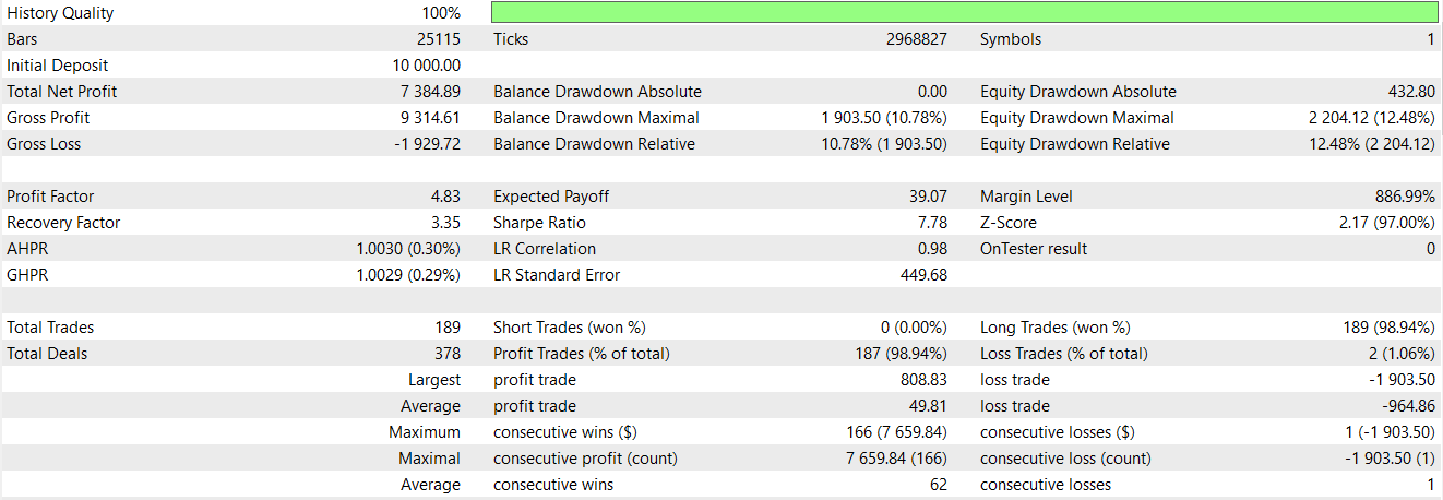
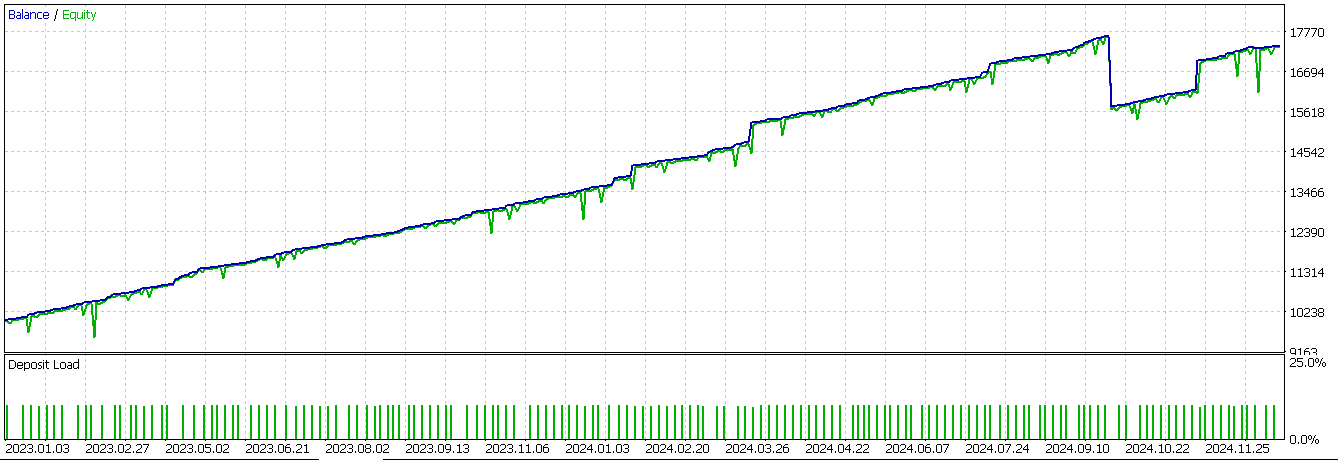
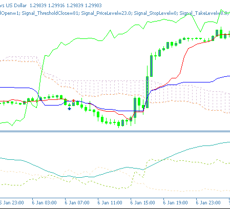
Our network, which overlays the last article signal processing as a filter, again appears to make a difference in the performance of the wizard assembled Expert Advisor. A bullish pattern on a bar chart can appear as follows for feature-1:

Feature-5

The final pattern we are retesting is the 6th, pattern-5. We implement this as follows in Python as follows:

def feature_5(df):
    """

    """
    feature = np.zeros((len(df), 2))
    
    feature[:, 0] = ((df['close'].shift(2) > df['close'].shift(1)) &
                     (df['close'].shift(1) < df['close']) &
                     (df['close'].shift(2) > df['Tenkan_sen'].shift(2)) &
                     (df['close'] > df['Tenkan_sen']) &
                     (df['close'].shift(1) <= df['Tenkan_sen'].shift(1)) &
                     (df['+DI'] > df['-DI']) &
                     (df['ADX'] >= 25.0)).astype(int)
    
    feature[:, 1] = ((df['close'].shift(2) < df['close'].shift(1)) &
                     (df['close'].shift(1) > df['close']) &
                     (df['close'].shift(2) < df['Tenkan_sen'].shift(2)) &
                     (df['close'] < df['Tenkan_sen']) &
                     (df['close'].shift(1) >= df['Tenkan_sen'].shift(1)) &
                     (df['+DI'] < df['-DI']) &
                     (df['ADX'] >= 25.0)).astype(int)
    
    
    feature[0, :] = 0
    feature[1, :] = 0
    
    return feature

Our format is similar to pattern-0 and pattern-1 above. In the way, we initialize and size our output NumPy array. To assign a 1 to the first column, affirming the bullish signal, we require: the close price buffer to deflect/bounce-off in a U turn over the Tenkan-sen. In addition, the plus DM should be above the minus DM with the ADX at 25 or more. This price action often signals a trend continuation and the relative size of the signed directional movement buffers of the ADX as well as its values all need to be considered before this is deemed the case.

The second column gets assigned a 1 to replace the default 0 if we have price deflecting on the Tenkan-sen from below such that the current close is presently below it, and the ADX is also at least 25 with the minus directional movement being more than the positive DM as a final signal confirmation. We conclude by turning to zero the first 2 rows of our feature array to cater for shift calculations that result in NaN values given the terminal nature of the input data. We tested this pattern as well in conditions similar to the other 2 patterns above, and we got the following report.

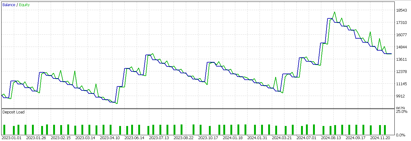
Our model is profitable, however the equity trajectory is very choppy. So there is a case for supplementing machine learning with typical indicator signals. While our results are not ideal and the testing is also limited, the case could be made that supplementing indicator signals with a spectral mixture kernel network can be done as an extra filter to sharpen trade entry and improve performance.

Conclusion

We have explored the use of a neural network designed after the spectral mixture kernel in fine-tuning the raw trade signals of the indicator pairing Ichimoku and ADX-Wilder. The special network we have adopted has shown some promise, and certainly a difference in performance to what we had in the last article, where trades were being placed solely with the indicator signals. Our results presented here, as always, require further diligence on the part of the reader before they can be adopted or incorporated into existing trade systems. The notion of incorporation, especially when testing, is something the MQL5 Wizard assembled Expert Advisors allow; since multiple custom signals can be selected during assembly.

name	description
WZ-74.mq5	Wizard assembled Expert Advisor whose header shows files used in assembly
SignalWZ-74.mqh	Custom signal class file
74-5.onnx	ONNX network for signal pattern-5
74-1.onnx	ONNX network for signal pattern-1
74-0.onnx	ONNX pattern for signal pattern-0