
Neural networks made easy (Part 60): Online Decision Transformer (ODT)

Introduction
The last two articles were devoted to the Decision Transformer method, which models action sequences in the context of an autoregressive model of desired rewards. As you might remember, according to the results of practical tests of two articles, the beginning of the testing period saw a fairly good increase in the profitability of the trained model results. Further on, the performance of the model decreases and a number of unprofitable transactions are observed, which leads to losses. The amount of losses received may exceed previously received profits.
The periodic additional training of the model can probably help here. However, this approach greatly complicates operating the model. So it is quite reasonable to consider the option of online model training. Here we are faced with a number of problems we have to solve.
One of the options for implementing Decision Transformer online training is presented in the article "Online Decision Transformer" (February 2022). It is worth noting that the proposed method uses primary offline training of classical DT. Online training is applied in the subsequent fine-tuning of the model. The experimental results presented in the author's article demonstrate that ODT is able to compete with the leaders in absolute performance on the D4RL test sample. Besides, it shows a much more significant improvement during the fine-tuning.
Let's look at the proposed method in the context of solving our problems.
1. ODT algorithm
Before considering the Online Decision Transformer algorithm, I propose to briefly recall the classic Decision Transformer. DT processes the τ trajectory as a sequence of several input tokens: Return-to-Go (RTG), states and actions. In particular, the initial RTG value is equal to the return for the entire trajectory. At the t temporary step, DT uses the tokens of the K last time steps to generate the At action. In this case, K is a hyperparameter that specifies the context length for the transformer. During the operation, the context length may be shorter than during training.
DT learns π(At|St, RTGt) deterministic policy, where St is a K sequence of the last states from t-K+1 to t. Similarly, RTGt personifies K last Return-to-Go. This is an auto regression model of K order. The Agent policy is trained to predict actions using a standard MSE (mean square error) loss function.
During operation, we indicate the desired performance of RTGinit and initial state S0. Then DT generates A0 action. After generating the At action, we execute it and observe the next state St+1 receiving the reward rt. This yields RTGt+1.
![]()
As before, DT generates A1 action based on the trajectory including A0, S0, S1 and RTG0, RTG1. This process is repeated until the episode is completed.
Policies trained only on offline datasets are usually suboptimal due to limited training set data. Offline trajectories may have low return and cover only a limited part of the state and action space. A natural strategy for improving performance is to further train RL Agents in online interaction with the environment. But the standard Decision Transformer method is not sufficient for online training.
The Online Decision Transformer algorithm introduces key modifications to Decision Transformer to ensure effective online training. The first step is a generalized probabilistic training goal. In this context, the goal is to train a stochastic policy that maximizes the probability of repeating a trajectory.
The main property of an online RL algorithm is its ability to balance exploration and exploitation. Even with stochastic policies, the traditional DT formulation does not take exploration into account. To solve this problem, the authors of the ODT method define the study through the entropy of the policy, which depends on the distribution of data in the trajectory. This distribution is static during offline pre-training, but dynamic during online setup as it depends on new data obtained during interaction with the environment.
Similar to many existing maximum entropy RL algorithms, such as Soft Actor Critic, the authors of the ODT method explicitly define a lower bound on policy entropy to encourage exploration.
The difference between the ODT loss function and SAC and other classical RL methods is that in ODT the loss function is a negative log likelihood rather than a discounted return. Basically, we focus only on training using a pattern of action sequences, instead of explicitly maximizing the return. And the objective function automatically adapts to the appropriate Actor policy in both offline and online training. During offline training, cross-entropy controls the degree of divergence of the distribution, while during online training it drives the exploration policy.
Another important difference from classical maximum entropy RL methods is that in ODT the policy entropy is defined at the level of sequences rather than transitions. While SAC imposes the β lower limit for policy entropy at all time steps, ODT limits the entropy to be averaged on K successive time steps. Thus, the constraint only requires that the entropy averaged over a sequence ofK time steps was higher than the specified β value. Therefore, any policy that satisfies the transition-level constraint also satisfies the sequence-level constraint. Thus, the feasible policy space is larger when K > 1. When K = 1, the sequence-level constraint is reduced to a transition-level constraint similar to SAC.
During model training, a replay buffer is used to record previous experience with periodic updates. For most existing RL algorithms, the experience rendering buffer consists of transitions. After each stage of online interaction within one epoch, the Agent's policy and Q-function are updated using gradient descent. The policy is then executed to collect new transitions and add them to the experience replay buffer. In case of ODT, the experience playback buffer consists of trajectories rather than transitions. After preliminary offline training, we initialize the experience playback buffer using trajectories with maximum results from the offline data set. Each time we interact with the environment, we fully execute the episode with the current policy. Then we update the experience playback buffer using the collected trajectory in FIFO order. Next, we update the Agent policy and execute a new episode. Evaluating policies using average actions typically results in higher rewards, but it is useful to use random actions for online research as it generates more diverse trajectories and behavioral patterns.
In addition, the ODT algorithm requires a hyperparameter in the form of an initial RTG to collect additional online data. Various works demonstrate that the actual estimated return of offline DT has a strong correlation with the initial RTG empirically and can often extrapolate RTG values beyond the maximum returns observed in the offline dataset. The ODT authors found that it is best to set this hyperparameter with a small fixed scaling from the existing expert results. The authors of the method use 2x scaling in their work. The original paper presents experimental results with much larger values, as well as ones that change during training (for example, quantiles of the best estimated return in offline and online datasets). But in practice they were not as effective as fixed scaled RTG.
Like DT, the ODT algorithm uses a two-step sampling procedure to ensure uniform sampling of sub-trajectories of K length in the playback buffer. First, we sample one trajectory with a probability proportional to its length. Then choose the K length sub-trajectory with equal probability.
We will get acquainted with the practical implementation of the method in the next section of the article.
2. Implementation using MQL5
After getting acquainted with the theoretical aspects of the method, let's move on to its practical implementation. This section will present our own vision of the implementation of the proposed approaches supplemented by developments from previous articles. In particular, the ODT algorithm includes two-stage model training:
- Preliminary offline training.
- Fine-tuning the model during online interaction with the environment.
For the purposes of this article, we will use the pre-trained model from the previous article. Therefore, we skip the first stage of offline training, which has already been carried out earlier and immediately move on to the second part of the model training.
It should also be noted here that when considering the DoC method in the previous article, we built and conducted offline training of two models:
- RTG generation;
- Actor's policy.
Using the RTG model generation is a departure from the original ODT algorithm, which proposes the use of expert assessment scaling for the initial RTG with subsequent adjustment of the goal to the actual results obtained.
In addition, using previously trained models does not allow us to change the architecture of the models. But let's see how the architecture of the models used corresponds to the ODT algorithm.
The authors of the method propose to use the stochastic Actor policy. This is the model we used in previous articles.
ODT proposes to use a trajectory experience replay buffer instead of individual trajectories. This is exactly the buffer we work with.
When training the models, we did not use the entropy component of the loss function to encourage environmental exploration. At this stage, we will not add it and accept the possible risks. We expect that the stochastic Actor policy and RTG generation model will provide sufficient exploration in the process of online interaction with the environment.
Another point that I excluded from my implementation concerns the experience playback buffer. After offline training, the authors of the method propose selecting a number of the most profitable trajectories that will be used in the first stages of online training. We initially limited the number of trajectories in the experience playback buffer. When moving to online training, we will use the entire existing experience reproduction buffer, to which we will add new trajectories in the process of interaction with the environment. At the same time, we will not immediately delete the oldest trajectories when adding new ones. We will limit the buffer size using previously created means when saving data to a file after completing the pass.
Thus, taking into account possible risks, we can easily use the models trained in the previous article. Then we will try to increase their efficiency by fine-tuning the process of online training of models using ODT approaches.
Here we have to resolve some constructive issues. The trading process is conditionally endless by its nature. I say "conditionally" because it is still finite for a number of reasons. But the probability of such an event occurring in the foreseeable future is so small that we consider it infinite. Consequently, we carry out the process of additional training not after the end of the episode, as suggested by the authors of the method, but with a certain frequency.
Here I would like to remind you that in our DT implementation, only the data of the last bar is supplied to the model input. The entire amount of historical data context is stored in the embedding layer's results buffer. This approach allowed us to reduce resource consumption for redundant data reprocessing. But this becomes one of the "stumbling blocks" on the path of online training. The fact is that the data in the embedding buffer is stored in strict historical sequence. Using the model in the process of periodic additional training leads to refilling the buffer with historical data from other trajectories or the same trajectory, but from a different segment of history. This distorts the data when continuing to interact with the environment after additional training of the models.
There are actually several options for solving this issue. All have varying implementation complexity and resource consumption during operation. At first glance, the simplest thing is to create a copy of the buffer and, before continuing the process of interaction with the environment, return the buffer to the state before starting the training. However, upon closer examination of the process, we understand that on the side of the main model, work is carried out only with the top-level class of the model without access to individual buffers of the neural layers. In this context, the simple process of copying the data of one buffer from the model and back into the model leads to a number of design changes. This significantly complicates the implementation of this method.
We can repeatedly transfer the entire set of historical data to the model after completing the additional training without making constructive changes to the model. But this leads to a significant amount of repetition of forward model pass operations. The volume of such operations grows as the size of the context increases. This makes the approach inefficient. The consumption of time and computing resources for data reprocessing can exceed the savings achieved by storing the history of embeddings in the neural layer buffer.
Another solution to the problem is to use duplicate models. One is needed for interaction with the environment. The second one is used in the additional training. This approach is more expensive in terms of memory resources, but completely solves the issue of data in the embedding layer buffer. But the question of data exchange between models arises. After all, after additional training, the model of interaction with the environment should use the updated Agent policy. The same goes for the RTG generation model. Here we can remember the Soft Actor-Critic method with its soft update of target models. Strange as it may seem, this is the mechanism that will allow us to transfer updated weighting ratios between models without changing the remaining buffers, including buffers of the embedding layer results.
To use this approach, we have to add a weight exchange method to the embedding layer, which was not previously used in the SAC implementation.
Here we should say that when adding a method, we make additions only directly to the CNeuronEmbeddingOCL class, since all the necessary APIs for its functioning have already been laid down by us earlier and implemented in the form of a virtual method of the base class of the CNeuronBaseOCL neural layer. It should also be noted that without making the specified modification, the operation of our model will not produce an error. After all, the method of the parent class will be used by default. But such work in this case will not be complete and correct.
To maintain consistency and correct overriding of virtual methods, we declare a method that saves parameters. In the method body, we immediately call a similar method of the parent class.
bool CNeuronEmbeddingOCL::WeightsUpdate(CNeuronBaseOCL *source, float tau)
  {
   if(!CNeuronBaseOCL::WeightsUpdate(source, tau))
      return false;
As we have said more than once, this approach of calling the parent class allows us to implement all the necessary controls in one action without unnecessary duplication and perform the necessary operations with inherited objects.
After successfully completing the operations of the parent class method, we move on to working on objects declared directly in our embedding class. But in order to gain access to similar objects of the donor class, we should override the type of the resulting object.
//---
   CNeuronEmbeddingOCL *temp = source;
Next we need to transfer the parameters of the WeightsEmbedding buffer. But before continuing operations, we will compare the buffer sizes of the current and donor objects.
   if(WeightsEmbedding.Total() != temp.WeightsEmbedding.Total())
      return false;
Then we have to transfer the content from one buffer to another. But we remember that all operations with buffers are performed on the OpenCL context side. Therefore, we will carry out data transfer on the context side. I deliberately use the "data transfer" phrase rather than "copying". I leave the possibility of "soft copying" with a ratio, as was provided for by the SAC algorithm for target models. OpenCL program kernels were created earlier. Now we only have to arrange their call.
We define the kernel task space in terms of the size of the weight ratio buffer.
   uint global_work_offset[1] = {0};
   uint global_work_size[1] = {WeightsEmbedding.Total()};
Next follows the branching of the algorithm depending on the parameter updating algorithm used. The branching is necessary because we will need more buffers and hyperparameters if we use the Adam method. This leads to the use of different kernels.
First we create the Adam method branch. To use it, two conditions should be met:
- specifying the appropriate method for updating parameters when creating an object, since the creation of objects of the corresponding data buffers depends on this;
- the update ratio should be different from one, otherwise a complete copy of the data is necessary, regardless of the parameter update method used.
   if(tau != 1.0f && optimization == ADAM)
     {
      if(!OpenCL.SetArgumentBuffer(def_k_SoftUpdateAdam, def_k_sua_target, WeightsEmbedding.GetIndex()))
        {
         printf("Error of set parameter kernel %s: %d; line %d", __FUNCTION__, GetLastError(), __LINE__);
         return false;
        }
      if(!OpenCL.SetArgumentBuffer(def_k_SoftUpdateAdam, def_k_sua_source, temp.WeightsEmbedding.GetIndex()))
        {
         printf("Error of set parameter kernel %s: %d; line %d", __FUNCTION__, GetLastError(), __LINE__);
         return false;
        }
      if(!OpenCL.SetArgumentBuffer(def_k_SoftUpdateAdam, def_k_sua_matrix_m, FirstMomentumEmbed.GetIndex()))
        {
         printf("Error of set parameter kernel %s: %d; line %d", __FUNCTION__, GetLastError(), __LINE__);
         return false;
        }
      if(!OpenCL.SetArgumentBuffer(def_k_SoftUpdateAdam, def_k_sua_matrix_v, SecondMomentumEmbed.GetIndex()))
        {
         printf("Error of set parameter kernel %s: %d; line %d", __FUNCTION__, GetLastError(), __LINE__);
         return false;
        }
      if(!OpenCL.SetArgument(def_k_SoftUpdateAdam, def_k_sua_tau, (float)tau))
        {
         printf("Error of set parameter kernel %s: %d; line %d", __FUNCTION__, GetLastError(), __LINE__);
         return false;
        }
      if(!OpenCL.SetArgument(def_k_SoftUpdateAdam, def_k_sua_b1, (float)b1))
        {
         printf("Error of set parameter kernel %s: %d; line %d", __FUNCTION__, GetLastError(), __LINE__);
         return false;
        }
      if(!OpenCL.SetArgument(def_k_SoftUpdateAdam, def_k_sua_b2, (float)b2))
        {
         printf("Error of set parameter kernel %s: %d; line %d", __FUNCTION__, GetLastError(), __LINE__);
         return false;
        }
      if(!OpenCL.Execute(def_k_SoftUpdateAdam, 1, global_work_offset, global_work_size))
        {
         printf("Error of execution kernel %s: %d", __FUNCTION__, GetLastError());
         return false;
        }
     }
Then we send the SoftUpdateAdam kernel to the execution queue.
We perform similar operations in the second branch of the algorithm, but for the SoftUpdate kernel.
   else
     {
      if(!OpenCL.SetArgumentBuffer(def_k_SoftUpdate, def_k_su_target, WeightsEmbedding.GetIndex()))
        {
         printf("Error of set parameter kernel %s: %d; line %d", __FUNCTION__, GetLastError(), __LINE__);
         return false;
        }
      if(!OpenCL.SetArgumentBuffer(def_k_SoftUpdate, def_k_su_source, temp.WeightsEmbedding.GetIndex()))
        {
         printf("Error of set parameter kernel %s: %d; line %d", __FUNCTION__, GetLastError(), __LINE__);
         return false;
        }
      if(!OpenCL.SetArgument(def_k_SoftUpdate, def_k_su_tau, (float)tau))
        {
         printf("Error of set parameter kernel %s: %d; line %d", __FUNCTION__, GetLastError(), __LINE__);
         return false;
        }
      if(!OpenCL.Execute(def_k_SoftUpdate, 1, global_work_offset, global_work_size))
        {
         printf("Error of execution kernel %s: %d", __FUNCTION__, GetLastError());
         return false;
        }
     }
//---
   return true;
  }
The constructive problem has been solved, and we can move on to the practical implementation of the online training method. We arrange the process of interaction with the environment and simultaneous additional training of models in the "...\DoC\OnlineStudy.mq5" EA. This EA is a kind of symbiosis of the EAs discussed in previous articles for collecting data for training and direct offline training of models. It contains all the external parameters necessary to interact with the environment, in particular, indicator parameters. But at the same time, we add parameters to indicate the frequency and number of iterations of online training. The default EA contains subjective data. I indicated the training frequency at 120 candles, which on the H1 timeframe approximately corresponds to 1 week (5 days * 24 hours). During the optimization, you can select values that will be more optimal for your models.
//+------------------------------------------------------------------+
//| Input parameters                                                 |
//+------------------------------------------------------------------+
input ENUM_TIMEFRAMES      TimeFrame   =  PERIOD_H1;
//---
input group                "---- RSI ----"
input int                  RSIPeriod   =  14;            //Period
input ENUM_APPLIED_PRICE   RSIPrice    =  PRICE_CLOSE;   //Applied price
//---
input group                "---- CCI ----"
input int                  CCIPeriod   =  14;            //Period
input ENUM_APPLIED_PRICE   CCIPrice    =  PRICE_TYPICAL; //Applied price
//---
input group                "---- ATR ----"
input int                  ATRPeriod   =  14;            //Period
//---
input group                "---- MACD ----"
input int                  FastPeriod  =  12;            //Fast
input int                  SlowPeriod  =  26;            //Slow
input int                  SignalPeriod=   9;            //Signal
input ENUM_APPLIED_PRICE   MACDPrice   =  PRICE_CLOSE;   //Applied price
//---
input int                  StudyIters  =   5;            //Iterations to Study
input int                  StudyPeriod =  120;           //Bars between Studies
In the EA initialization method, we first upload the previously created experience playback buffer. We performed similar actions in the "Study.mql5" training EAs for various offline training methods. Only now we do not terminate the EA if data loading fails. Unlike the offline mode, we allow models to be trained only on new data that will be collected when interacting with the environment.
//+------------------------------------------------------------------+
//| Expert initialization function                                   |
//+------------------------------------------------------------------+
int OnInit()
  {
   LoadTotalBase();
Next, we will prepare indicators, just as we did earlier in the EAs for interaction with the environment.
   if(!Symb.Name(_Symbol))
      return INIT_FAILED;
   Symb.Refresh();
//---
   if(!RSI.Create(Symb.Name(), TimeFrame, RSIPeriod, RSIPrice))
      return INIT_FAILED;
//---
   if(!CCI.Create(Symb.Name(), TimeFrame, CCIPeriod, CCIPrice))
      return INIT_FAILED;
//---
   if(!ATR.Create(Symb.Name(), TimeFrame, ATRPeriod))
      return INIT_FAILED;
//---
   if(!MACD.Create(Symb.Name(), TimeFrame, FastPeriod, SlowPeriod, SignalPeriod, MACDPrice))
      return INIT_FAILED;
   if(!RSI.BufferResize(NBarInPattern) || !CCI.BufferResize(NBarInPattern) ||
      !ATR.BufferResize(NBarInPattern) || !MACD.BufferResize(NBarInPattern))
     {
      PrintFormat("%s -> %d", __FUNCTION__, __LINE__);
      return INIT_FAILED;
     }
//---
   if(!Trade.SetTypeFillingBySymbol(Symb.Name()))
      return INIT_FAILED;
Let's load the models and check their compliance in terms of the sizes of the source data layers and the results. If necessary, we create new models with a predefined architecture. This goes a bit beyond the scope of additional training of models. But we leave the opportunity for the user to carry out online training "from scratch".
//--- load models
   float temp;
   if(!Agent.Load(FileName + "Act.nnw", temp, temp, temp, dtStudied, true) ||
      !RTG.Load(FileName + "RTG.nnw", dtStudied, true) ||
      !AgentStudy.Load(FileName + "Act.nnw", temp, temp, temp, dtStudied, true) ||
      !RTGStudy.Load(FileName + "RTG.nnw", dtStudied, true))
     {
      PrintFormat("Can't load pretrained models");
      CArrayObj *agent = new CArrayObj();
      CArrayObj *rtg = new CArrayObj();
      if(!CreateDescriptions(agent, rtg))
        {
         delete agent;
         delete rtg;
         PrintFormat("Can't create description of models");
         return INIT_FAILED;
        }
      if(!Agent.Create(agent) ||
         !RTG.Create(rtg) ||
         !AgentStudy.Create(agent) ||
         !RTGStudy.Create(rtg))
        {
         delete agent;
         delete rtg;
         PrintFormat("Can't create models");
         return INIT_FAILED;
        }
      delete agent;
      delete rtg;
      //---
     }
//---
   Agent.getResults(Result);
   if(Result.Total() != NActions)
     {
      PrintFormat("The scope of the actor does not match the actions count (%d <> %d)", NActions, Result.Total());
      return INIT_FAILED;
     }
   AgentResult = vector<float>::Zeros(NActions);
//---
   Agent.GetLayerOutput(0, Result);
   if(Result.Total() != (NRewards + BarDescr * NBarInPattern + AccountDescr + TimeDescription + NActions))
     {
      PrintFormat("Input size of Actor doesn't match state description (%d <> %d)",
           Result.Total(), (NRewards + BarDescr * NBarInPattern + AccountDescr + TimeDescription + NActions));
      return INIT_FAILED;
     }
   Agent.Clear();
   RTG.Clear();
Please note that we are loading (or initializing) two copies of each model. One is needed for interaction with the environment. The second is used in training. The trained models received the Study suffix.
Next, we initialize global variables and terminate the method.
   PrevBalance = AccountInfoDouble(ACCOUNT_BALANCE);
   PrevEquity = AccountInfoDouble(ACCOUNT_EQUITY);
//---
   return(INIT_SUCCEEDED);
  }
In the EA deinitialization method, we save the trained models and the accumulated experience reproduction buffer.
//+------------------------------------------------------------------+
//| Expert deinitialization function                                 |
//+------------------------------------------------------------------+
void OnDeinit(const int reason)
  {
//---
   AgentStudy.Save(FileName + "Act.nnw", 0, 0, 0, TimeCurrent(), true);
   RTGStudy.Save(FileName + "RTG.nnw", TimeCurrent(), true);
   delete Result;
   int total = ArraySize(Buffer);
   printf("Saving %d", MathMin(total + 1, MaxReplayBuffer));
   SaveTotalBase();
   Print("Saved");
  }
Please note that we save the trained models since their buffers contain all the information necessary for subsequent training and operation of the models.
The process of interaction with the environment is arranged in the OnTick tick processing method. At the beginning of the method, we check for the occurrence of a new bar opening event and, if necessary, update the indicator parameters. We also download price movement data.
//+------------------------------------------------------------------+
//| Expert tick function                                             |
//+------------------------------------------------------------------+
void OnTick()
  {
//---
   if(!IsNewBar())
      return;
//---
   int bars = CopyRates(Symb.Name(), TimeFrame, iTime(Symb.Name(), TimeFrame, 1), NBarInPattern, Rates);
   if(!ArraySetAsSeries(Rates, true))
      return;
//---
   RSI.Refresh();
   CCI.Refresh();
   ATR.Refresh();
   MACD.Refresh();
   Symb.Refresh();
   Symb.RefreshRates();
Prepare the data received from the terminal for transmission to the model of interaction with the environment as input data.
//--- History data
   float atr = 0;
   for(int b = 0; b < (int)NBarInPattern; b++)
     {
      float open = (float)Rates[b].open;
      float rsi = (float)RSI.Main(b);
      float cci = (float)CCI.Main(b);
      atr = (float)ATR.Main(b);
      float macd = (float)MACD.Main(b);
      float sign = (float)MACD.Signal(b);
      if(rsi == EMPTY_VALUE || cci == EMPTY_VALUE || atr == EMPTY_VALUE || macd == EMPTY_VALUE || sign == EMPTY_VALUE)
         continue;
      //---
      int shift = b * BarDescr;
      sState.state[shift] = (float)(Rates[b].close - open);
      sState.state[shift + 1] = (float)(Rates[b].high - open);
      sState.state[shift + 2] = (float)(Rates[b].low - open);
      sState.state[shift + 3] = (float)(Rates[b].tick_volume / 1000.0f);
      sState.state[shift + 4] = rsi;
      sState.state[shift + 5] = cci;
      sState.state[shift + 6] = atr;
      sState.state[shift + 7] = macd;
      sState.state[shift + 8] = sign;
     }
   bState.AssignArray(sState.state);
Let's supplement the data buffer with information about the account status.
//--- Account description
   sState.account[0] = (float)AccountInfoDouble(ACCOUNT_BALANCE);
   sState.account[1] = (float)AccountInfoDouble(ACCOUNT_EQUITY);
//---
   double buy_value = 0, sell_value = 0, buy_profit = 0, sell_profit = 0;
   double position_discount = 0;
   double multiplyer = 1.0 / (60.0 * 60.0 * 10.0);
   int total = PositionsTotal();
   datetime current = TimeCurrent();
   for(int i = 0; i < total; i++)
     {
      if(PositionGetSymbol(i) != Symb.Name())
         continue;
      double profit = PositionGetDouble(POSITION_PROFIT);
      switch((int)PositionGetInteger(POSITION_TYPE))
        {
         case POSITION_TYPE_BUY:
            buy_value += PositionGetDouble(POSITION_VOLUME);
            buy_profit += profit;
            break;
         case POSITION_TYPE_SELL:
            sell_value += PositionGetDouble(POSITION_VOLUME);
            sell_profit += profit;
            break;
        }
      position_discount += profit - (current - PositionGetInteger(POSITION_TIME)) * multiplyer * MathAbs(profit);
     }
   sState.account[2] = (float)buy_value;
   sState.account[3] = (float)sell_value;
   sState.account[4] = (float)buy_profit;
   sState.account[5] = (float)sell_profit;
   sState.account[6] = (float)position_discount;
   sState.account[7] = (float)Rates[0].time;
//---
   bState.Add((float)((sState.account[0] - PrevBalance) / PrevBalance));
   bState.Add((float)(sState.account[1] / PrevBalance));
   bState.Add((float)((sState.account[1] - PrevEquity) / PrevEquity));
   bState.Add(sState.account[2]);
   bState.Add(sState.account[3]);
   bState.Add((float)(sState.account[4] / PrevBalance));
   bState.Add((float)(sState.account[5] / PrevBalance));
   bState.Add((float)(sState.account[6] / PrevBalance));
Next, create a timestamp.
//--- Time label
   double x = (double)Rates[0].time / (double)(D'2024.01.01' - D'2023.01.01');
   bState.Add((float)MathSin(2.0 * M_PI * x));
   x = (double)Rates[0].time / (double)PeriodSeconds(PERIOD_MN1);
   bState.Add((float)MathCos(2.0 * M_PI * x));
   x = (double)Rates[0].time / (double)PeriodSeconds(PERIOD_W1);
   bState.Add((float)MathSin(2.0 * M_PI * x));
   x = (double)Rates[0].time / (double)PeriodSeconds(PERIOD_D1);
   bState.Add((float)MathSin(2.0 * M_PI * x));
Add the vector of the Agent’s latest actions that led us to the current state.
//--- Prev action
   bState.AddArray(AgentResult);
The collected data is sufficient to perform a forward pass of the RTG generation model.
//--- Return to go
   if(!RTG.feedForward(GetPointer(bState)))
      return;
In fact, our vector of initial data only lacks this data to predict the Agent’s optimal actions in the current time period. Therefore, after a successful forward pass of the first model, we add the obtained results to the source data buffer and call the forward pass method of our Actor. Make sure to check the results of the operations.
   RTG.getResults(Result);
   bState.AddArray(Result);
//---
   if(!Agent.feedForward(GetPointer(bState), 1, false, (CBufferFloat*)NULL))
      return;
After successfully performing a forward pass through the models, we will decipher the results of their work and perform the selected action in the environment. This process is fully consistent with the previously discussed algorithm in models of interaction with the environment.
//---
   PrevBalance = sState.account[0];
   PrevEquity = sState.account[1];
//---
   vector<float> temp;
   Agent.getResults(temp);
//---
   double min_lot = Symb.LotsMin();
   double step_lot = Symb.LotsStep();
   double stops = MathMax(Symb.StopsLevel(), 1) * Symb.Point();
   if(temp[0] >= temp[3])
     {
      temp[0] -= temp[3];
      temp[3] = 0;
     }
   else
     {
      temp[3] -= temp[0];
      temp[0] = 0;
     }
   float delta = MathAbs(AgentResult - temp).Sum();
   AgentResult = temp;
//--- buy control
   if(temp[0] < min_lot || (temp[1] * MaxTP * Symb.Point()) <= stops || (temp[2] * MaxSL * Symb.Point()) <= stops)
     {
      if(buy_value > 0)
         CloseByDirection(POSITION_TYPE_BUY);
     }
   else
     {
      double buy_lot = min_lot + MathRound((double)(temp[0] - min_lot) / step_lot) * step_lot;
      double buy_tp = Symb.NormalizePrice(Symb.Ask() + temp[1] * MaxTP * Symb.Point());
      double buy_sl = Symb.NormalizePrice(Symb.Ask() - temp[2] * MaxSL * Symb.Point());
      if(buy_value > 0)
         TrailPosition(POSITION_TYPE_BUY, buy_sl, buy_tp);
      if(buy_value != buy_lot)
        {
         if(buy_value > buy_lot)
            ClosePartial(POSITION_TYPE_BUY, buy_value - buy_lot);
         else
            Trade.Buy(buy_lot - buy_value, Symb.Name(), Symb.Ask(), buy_sl, buy_tp);
        }
     }
//--- sell control
   if(temp[3] < min_lot || (temp[4] * MaxTP * Symb.Point()) <= stops || (temp[5] * MaxSL * Symb.Point()) <= stops)
     {
      if(sell_value > 0)
         CloseByDirection(POSITION_TYPE_SELL);
     }
   else
     {
      double sell_lot = min_lot + MathRound((double)(temp[3] - min_lot) / step_lot) * step_lot;;
      double sell_tp = Symb.NormalizePrice(Symb.Bid() - temp[4] * MaxTP * Symb.Point());
      double sell_sl = Symb.NormalizePrice(Symb.Bid() + temp[5] * MaxSL * Symb.Point());
      if(sell_value > 0)
         TrailPosition(POSITION_TYPE_SELL, sell_sl, sell_tp);
      if(sell_value != sell_lot)
        {
         if(sell_value > sell_lot)
            ClosePartial(POSITION_TYPE_SELL, sell_value - sell_lot);
         else
            Trade.Sell(sell_lot - sell_value, Symb.Name(), Symb.Bid(), sell_sl, sell_tp);
        }
     }
Evaluate the reward from the environment for the transition to the current state. Transmit all the collected information to form the current trajectory.
//---
   int shift = BarDescr * (NBarInPattern - 1);
   sState.rewards[0] = bState[shift];
   sState.rewards[1] = bState[shift + 1] - 1.0f;
   if((buy_value + sell_value) == 0)
      sState.rewards[2] -= (float)(atr / PrevBalance);
   else
      sState.rewards[2] = 0;
   for(ulong i = 0; i < NActions; i++)
      sState.action[i] = AgentResult[i];
   if(!Base.Add(sState))
      ExpertRemove();
This completes the process of interaction with the environment. But before exiting the method, we will check the need to start the process of additional training of models. I probably used the simplest control to test the method efficiency. I simply check the multiplicity of the size of the overall history for the instrument in the analyzed timeframe of the training period. In everyday work, it is advisable to use more thoughtful approaches to shift the additional training to periods of market closure or reduction in instrument volatility. In addition, it may be useful to delay updating model parameters until all positions have been closed. In general, for use in real models, I would recommend a more balanced and meaningful approach to the choice of frequency and time for additional training of models.
//---
   if((Bars(_Symbol, TimeFrame) % StudyPeriod) == 0)
      Train();
  }
Next, we turn our attention to the Train model training method. It should be noted here that additional training is carried out taking into account the experience gained in the process of current interaction with the environment. In the tick processing method, we collected all the information received from the environment into a separate trajectory. However, this trajectory is not added to the experience playback buffer. Previously, we carried out such an operation only after the end of the episode. But this approach is not acceptable in the case of periodic updating of parameters. After all, it brings us closer to offline training, when the Agent’s policy is trained only on fixed trajectories of previous experience. Therefore, before starting training, we will add the collected data to the experience replay buffer.
In order to prevent recording too short and uninformative trajectories, we will limit the minimum size of the saved trajectory. In the example given, I limited the minimum size of the trajectory during the update period of the model parameters.
If the size of the accumulated trajectory meets the minimum requirements, then we add it to the experience playback buffer and recalculate the cumulative amount of rewards.
Here it should be noted that we recalculate the cumulative amount of rewards only for the copy of the trajectory transferred to the experience playback buffer. In the initial buffer for accumulating information about the current trajectory, the reward should remain uncounted. With subsequent interaction with the environment, the trajectory will be supplemented. Therefore, with further addition of the updated trajectory, repeated recalculation of the cumulative reward will lead to doubling of the data. To prevent this, we always keep the non-recalculated reward in the trajectory accumulation buffer.
//+------------------------------------------------------------------+
//| Train function                                                   |
//+------------------------------------------------------------------+
void Train(void)
  {
   int total_tr = ArraySize(Buffer);
   if(Base.Total >= StudyPeriod)
      if(ArrayResize(Buffer, total_tr + 1) == (total_tr + 1))
        {
         Buffer[total_tr] = Base;
         Buffer[total_tr].CumRevards();
         total_tr++;
        }
Next, we should remember that the size of the trajectory accumulation buffer is limited by the Buffer_Size constant. In order to prevent an error of going beyond the array limits, make sure that there are sufficient free cells in the trajectory accumulation buffer to record steps until the next saving of the trajectory. Delete some of the oldest steps if necessary.
Please note that we are deleting data in the primary trajectory accumulation buffer. At the same time, this information is saved in the copy of the trajectory that we saved to the experience playback buffer.
When specifying model constants and parameters, we should make sure that the size of the trajectory buffer allows saving the history of at least one period between additional training of models.
   int clear = Base.Total + StudyPeriod - Buffer_Size;
   if(clear > 0)
      Base.ClearFirstN(clear);
Then I added one more additional control, which may seem unnecessary. I check the experience playback buffer for short trajectories and, if found, delete them. At first glance, the presence of such trajectories is unlikely due to the presence of similar control before adding the trajectory to the experience reproduction buffer. But I still admit the possibility of some failures when reading and writing trajectories to a file. We perform this check to eliminate subsequent errors.
//---
   int count = 0;
   for(int i = 0; i < (total_tr + count); i++)
     {
      if(Buffer[i + count].Total < StudyPeriod)
        {
         count++;
         i--;
         continue;
        }
      if(count > 0)
         Buffer[i] = Buffer[i + count];
     }
   if(count > 0)
     {
      ArrayResize(Buffer, total_tr - count);
      total_tr = ArraySize(Buffer);
     }
Next, we arrange a system of model training cycles. This process largely repeats the one from the previous article. The external loop is organized according to the number of model training iterations specified in the EA external parameters.
In the body of the loop, we randomly select a trajectory and an element of this trajectory, from which we will begin the next iteration of model training.
   uint ticks = GetTickCount();
//---
   bool StopFlag = false;
   for(int iter = 0; (iter < StudyIters && !IsStopped() && !StopFlag); iter ++)
     {
      int tr = (int)((MathRand() / 32767.0) * (total_tr - 1));
      int i = (int)((MathRand() * MathRand() / MathPow(32767, 2)) * MathMax(Buffer[tr].Total - 2 * HistoryBars,
                                                                            MathMin(Buffer[tr].Total, 20)));
      if(i < 0)
        {
         iter--;
         continue;
        }
Then we will clear the model embedding buffers and the vector of previous Actor actions.
      vector<float> Actions = vector<float>::Zeros(NActions);
      AgentStudy.Clear();
      RTGStudy.Clear();
At this stage, we have completed the preparatory work and can start training the models. Arrange a nested learning loop.
In the body of the loop, we repeat the process of preparing the source data buffer, similar to the one described above in the tick processing method. The sequence of writing data to the buffer is completely repeated. However, while we previously requested data from the terminal, now we take it from the experience playback buffer.
      for(int state = i; state < MathMin(Buffer[tr].Total - 2, int(i + HistoryBars * 1.5)); state++)
        {
         //--- History data
         bState.AssignArray(Buffer[tr].States[state].state);
         //--- Account description
         float prevBalance = (state == 0 ? Buffer[tr].States[state].account[0] : Buffer[tr].States[state - 1].account[0]);
         float prevEquity = (state == 0 ? Buffer[tr].States[state].account[1] : Buffer[tr].States[state - 1].account[1]);
         bState.Add((Buffer[tr].States[state].account[0] - prevBalance) / prevBalance);
         bState.Add(Buffer[tr].States[state].account[1] / prevBalance);
         bState.Add((Buffer[tr].States[state].account[1] - prevEquity) / prevEquity);
         bState.Add(Buffer[tr].States[state].account[2]);
         bState.Add(Buffer[tr].States[state].account[3]);
         bState.Add(Buffer[tr].States[state].account[4] / prevBalance);
         bState.Add(Buffer[tr].States[state].account[5] / prevBalance);
         bState.Add(Buffer[tr].States[state].account[6] / prevBalance);
         //--- Time label
         double x = (double)Buffer[tr].States[state].account[7] / (double)(D'2024.01.01' - D'2023.01.01');
         bState.Add((float)MathSin(2.0 * M_PI * x));
         x = (double)Buffer[tr].States[state].account[7] / (double)PeriodSeconds(PERIOD_MN1);
         bState.Add((float)MathCos(2.0 * M_PI * x));
         x = (double)Buffer[tr].States[state].account[7] / (double)PeriodSeconds(PERIOD_W1);
         bState.Add((float)MathSin(2.0 * M_PI * x));
         x = (double)Buffer[tr].States[state].account[7] / (double)PeriodSeconds(PERIOD_D1);
         bState.Add((float)MathSin(2.0 * M_PI * x));
         //--- Prev action
         bState.AddArray(Actions);
After collecting the first part of the initial data, we perform a forward pass of the RTG generation model. Then we immediately carry out a direct pass in order to minimize the error to the actual reward received. Thus, we build an autoregressive model for predicting possible rewards based on the previous trajectory of state and actions.
         //--- Return to go
         if(!RTGStudy.feedForward(GetPointer(bState)))
           {
            PrintFormat("%s -> %d", __FUNCTION__, __LINE__);
            StopFlag = true;
            break;
           }
         Result.AssignArray(Buffer[tr].States[state + 1].rewards);
         if(!RTGStudy.backProp(Result))
           {
            PrintFormat("%s -> %d", __FUNCTION__, __LINE__);
            StopFlag = true;
            break;
           }
For the purposes of training the Agent's policy, we indicate the actual reward received in the source data buffer, instead of the predictive RTG, and perform a direct pass.
         //--- Policy Feed Forward
         bState.AddArray(Buffer[tr].States[state + 1].rewards);
         if(!AgentStudy.feedForward(GetPointer(bState), 1, false, (CBufferFloat*)NULL))
           {
            PrintFormat("%s -> %d", __FUNCTION__, __LINE__);
            StopFlag = true;
            break;
           }
The Agent's policy is trained to minimize the error between the predicted and actually carried out action, which led to the receipt of the reward.
         //--- Policy study
         Actions.Assign(Buffer[tr].States[state].action);
         vector<float> result;
         AgentStudy.getResults(result);
         Result.AssignArray(CAGrad(Actions - result) + result);
         if(!AgentStudy.backProp(Result, (CBufferFloat*)NULL))
           {
            PrintFormat("%s -> %d", __FUNCTION__, __LINE__);
            StopFlag = true;
            break;
           }
This allows us to build an autoregressive model for selecting the optimal action to obtain the desired reward in the context of previously visited states and completed actions of the Agent.
After successfully completing the model training iterations, we inform the user about the progress of the training operations and move on to the next iteration of the model training loop.
Upon completion of all iterations of the system of nested loops of the model training process, we clear the comments field on the graph and transfer the parameters from the trained models to the environment interaction models. In the example above, I completely copy the weighting coefficient data. Thus, I emulate the use of one model for training and operation. However, I also allow experiments with different data copying ratios.
   Comment("");
//---
   Agent.WeightsUpdate(GetPointer(AgentStudy), 1.0f);
   RTG.WeightsUpdate(GetPointer(RTGStudy), 1.0f);
//---
  }
This concludes the solution transformer online training EA algorithm. Find the full EA code and all its methods in the attachment.
Please note that the "...\DoC\OnlineStudy.mq5" EA is located in the "DoC" subdirectory with the EAs from the previous article. I have not separated it into a separate subdirectory, since functionally it carries out additional training of models trained by offline EAs from the previous article. This way we maintain the integrity of the set of model training files.
You can also find all the programs used in both the current and previous articles in the attachment.
3. Test
We examined the theoretical aspects of the Online Decision Transformer method and built our own interpretation of the proposed method. The next stage is testing the work done. In fact, we fine-tune the models from the previous article. For these purposes, we carry out a cycle of single runs of our new EA on the history of training data in the strategy tester.
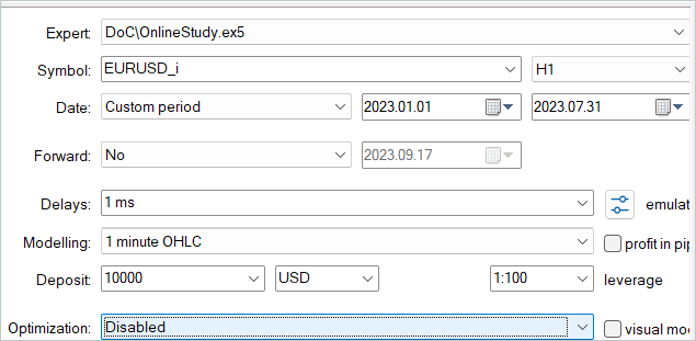
In the previous article, we carried out offline training of models on historical data for the first 7 months of 2023. It is during this same historical period that we fine-tune the models.
Through the process of fine-tuning the models, ODT improved the overall profitability of the models. On the test sample for August 2023, the model was able to earn about 10% profit. The yield chart is not perfect, but some trends are already visible on it.

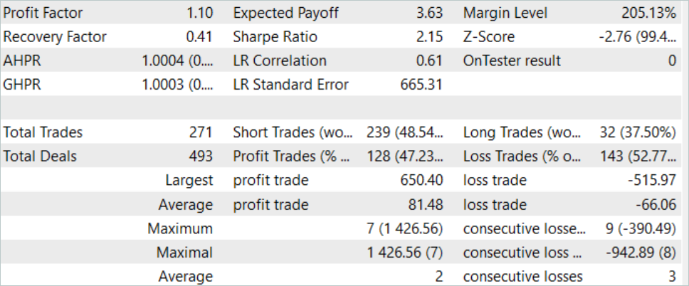
The results of testing the trained model are presented above. In total, 271 transactions were made during the test period. 128 of them were closed with a profit, which amounted to more than 47%. As we can see, the share of profitable trades is slightly less than losing ones. But the maximum profitable trade is 26% greater than the maximum loss. The average profitable trade is more than 20% higher than the average losing trade. All this allowed increasing the profit factor of the model to 1.10.
Conclusion
In this article, we continued to consider options for increasing the efficiency of the Decision Transformer method and got acquainted with the algorithm for fine-tuning models in Online Decision Transformer (ODT) training mode. This method allows increasing the efficiency of models trained offline and allows Agents to adapt to a changing environment, thereby improving their policies through interaction with the environment.
In the practical part of the article, we implemented the method using MQL5 and carried out online training of the models from the previous article. It is worth noting here that the optimization of the models was obtained only through the use of the considered ODT method. During the online training, we used models that were trained offline in the previous article. We have not implemented any design changes to the model architecture. Only additional online training has been provided. This made it possible to increase the efficiency of the models, which in itself confirms the efficiency of using the Online Decision Transformer method.
Once again, I would like to remind you that all the programs presented in the article are intended only to demonstrate the technology and are not ready for use in real trading.
Links
- Decision Transformer: Reinforcement Learning via Sequence Modeling
- Online Decision Transformer
- Dichotomy of Control: Separating What You Can Control from What You Cannot
- Neural networks made easy (Part 34): Fully parameterized quantile function
- Neural networks made easy (Part 58): Decision Transformer (DT)
- Neural networks are easy (Part 59): Dichotomy of Control (DoC)
Programs used in the article
| # | Name | Type | Description |
|---|---|---|---|
| 1 | Research.mq5 | Expert Advisor | Example collection EA |
| 2 | Study.mq5 | Expert Advisor | Agent training EA |
| 3 | OnlineStudy.mq5 | Expert Advisor | EA for agent additional online training |
| 4 | Test.mq5 | Expert Advisor | Model testing EA |
| 5 | Trajectory.mqh | Class library | System state description structure |
| 6 | NeuroNet.mqh | Class library | A library of classes for creating a neural network |
| 7 | NeuroNet.cl | Code Base | OpenCL program code library |
Translated from Russian by MetaQuotes Ltd.
Original article: https://www.mql5.com/ru/articles/13596
Warning: All rights to these materials are reserved by MetaQuotes Ltd. Copying or reprinting of these materials in whole or in part is prohibited.
This article was written by a user of the site and reflects their personal views. MetaQuotes Ltd is not responsible for the accuracy of the information presented, nor for any consequences resulting from the use of the solutions, strategies or recommendations described.

 Experiments with neural networks (Part 7): Passing indicators
- Free trading apps
- Over 8,000 signals for copying
- Economic news for exploring financial markets
You agree to website policy and terms of use