
Neural networks are easy (Part 59): Dichotomy of Control (DoC)

Introduction
The financial markets industry is a complex and multifaceted environment. Every event and action have their roots in economic fundamental processes. The reason for certain events can be found in the news, geopolitical events, various technical aspects and many other factors. Quite often, we observe such dependencies after they happen. While analyzing the market situation, we observe only a small part of these factors. This in general makes financial markets a rather difficult environment to analyze. But still, we highlight some of the most significant tools that can detect the main trends. Other factors are attributed to environmental stochasticity.
In such a complex environment, reinforcement learning represents a powerful tool for developing strategies in financial markets. However, existing methods, such as Decision Transformer, may not be adaptive enough in highly stochastic environments. This is what we observed in the practical part of the previous article.
As you might remember, unlike traditional methods, Decision Transformer models action sequences in the context of an autoregressive model of desired rewards. While training the model, a relationship is built between the sequence of states, actions, desired rewards and the actual result obtained from the environment. However, a large number of random factors can lead to a discrepancy between the trained strategy and the desired future outcome.
Many methods of reinforcement learning and others face a similar problem. In October 2022, the Google team presented the Dichotomy of Control method as one of the options for solving this issue.
1. DoC Method Basics
The dichotomy of control is the logical basis of Stoicism. It implies an understanding that everything that exists around us can be divided into two parts. The first one is subject to us and is completely under our control. We have no control over the second one and events will happen regardless of our actions.
We are working with the first area, while taking the second one for granted.
The authors of the "Dichotomy of Control" method implemented similar postulates into their algorithm. DoC allows us to separate what is under the control of strategy (action policy) and what is beyond its control (environmental stochasticity).
But before moving on to studying the method, I propose to remember how we represented the trajectory in DT.

Here R1 ("Return to go") represents our desire and is not related to the initial S0 state. Our trained model selects the action that produced the desired result on the training set. But the probability of obtaining the desired reward from the current state may be so small that the Agent’s actions will be far from optimal.
Now let's look at the world with our eyes wide open. In this context, "Return to go" is an instruction to the Agent to choose a behavior strategy. Don't you think it is similar to a skill in hierarchical models or target designation in GCRL. Probably, similar thoughts visited the authors of the DoC method, and they proposed using some kind of hidden state z(τ). But, as you know, substituting concepts does not change the essence. A training model is introduced to represent the z(τ) latent state.
The key observation of the method authors is that z should not contain information related to environmental stochasticity. It should not include information about the future Rt and St+1, which is unknown at the time of the previous history. Accordingly, a conditional restriction of mutual information between z and each Rt and St+1 pair in future is added to the goal. We will use contrast training methods to satisfy this mutual information constraint.
Next we introduce the conditional distribution ω(rt|τ0:t-1,st,at) parameterized by the f energy function.
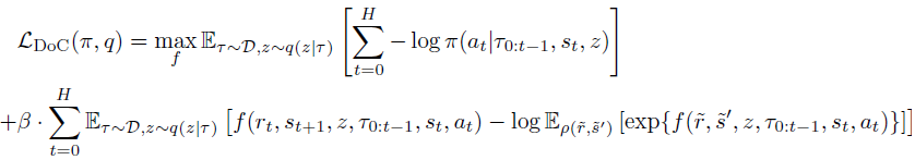
Combining this through the Lagrange ratios, we can train π and z(τ) by minimizing the end goal of DoC:
When applied to the Decision Transformer method, the DoC-trained policy requires a suitable z condition. To select the desired z associated with high expected reward, the authors of the method suggest:
- Select a large number of potential z values;
- Estimate the expected reward for each of these values of z;
- Select z with the highest expected reward and pass it to the policy.
To ensure such a procedure during the operational phase, two additional components are added to the method formulation. First, the prior distribution p(z|s0) a large number of z values are selected from. Second, the V(z) value function, which is used to rank potential z values. These components are trained by minimizing the following objective:

Note the use of stop-gradient to q(z|τ) when training p to avoid the q regularization relative to the prior distribution.
The article "Dichotomy of Control: Separating What You Can Control from What You Cannot" features quite a few examples demonstrating the significant superiority of the proposed method in various stochastic environments.
This is a rather interesting point, and I propose to test in practice the possibility of using this approach to solve our problems.
2. Implementation using MQL5
In the practical part of the article, we will consider the implementation of the Dichotomy of Control algorithm using MQL5. I would like to immediately draw your attention to the fact that the implementation in question is a personal interpretation of the proposed method. In some moments, it will be quite far from the original solution.
First of all, this implementation is a logical continuation of the programs from the previous article. We implement the proposed mechanisms into the previously created DT code in an attempt to optimize the model performance and increase its efficiency.
Moreover, we will try to simplify the DoC algorithm a little while maintaining the fundamental ideas.
As mentioned above, the authors of the method introduce some latent state instead of return-to-go. During the operation, a certain package of such latent states is sampled from the prior distribution p(z|s0). These latent states are subsequently estimated using the V(z) value function. In practice, this means that we extract the most similar states from the training set and select the latent representation with the highest expected reward. Consistent with the ideas of the control dichotomy, we consider not only the absolute value of the reward, but also the probability of receiving it.
Naturally, we will not go through the entire training set every time. Instead, we will use pre-trained models that approximate the corresponding features from the training set. But in any case, sampling a large number of latent representations and then estimating them is a rather labor-intensive task. Can we somehow simplify it?
Let's look at the essence of these entities. The z latent representation in the Decision Transformer context is the expected reward. So the value function V(z) may be a reflection of the z latent state itself. We might think about excluding the value function as a class and directly compare latent states with each other, but we will not take such a step.
Upon thinking about this further, the prior distribution p(z|s0) can be represented as a probabilistic distribution of the use of a particular latent representation in a specific environmental state. Let's recall the fully parameterized quantile function (FQF). It allows you to combine probability and quantitative distributions. This is what we will use in the latent representation generation model.
This solution allows us to combine the prior distribution and the cost function. Moreover, this way we can avoid sampling a batch of latent states and then estimating them.
We do the same with the ω(rt|τ0:t-1,st,at) conditional distribution parameterized by the f energy function.
Note that in both cases, we are generating a latent representation. In order to save resources, we will create two models and use one in both cases. Here we should remember that ω(rt|τ0:t-1,st,at) depends on the trajectory. Consequently, when constructing a model, we should take into account its autoregressive nature similar to the DT Actor model.
The architecture of both models is described in the CreateDescriptions method. In the method parameters, we pass pointers to two dynamic arrays to describe model architectures. The differences in the model architectures will not be significant. But they still exist. That is why we create two separate architectures, and not a common one. First, we create the architecture of the Actor model. Just as in the previous article, the source data layer contains only variable components of the environmental state (one bar data).
bool CreateDescriptions(CArrayObj *agent, CArrayObj *rtg)
  {
//---
   CLayerDescription *descr;
//---
   if(!agent)
     {
      agent = new CArrayObj();
      if(!agent)
         return false;
     }
//--- Agent
   agent.Clear();
//--- Input layer
   if(!(descr = new CLayerDescription()))
      return false;
   descr.type = defNeuronBaseOCL;
   int prev_count = descr.count = (NRewards + BarDescr*NBarInPattern + AccountDescr + TimeDescription + NActions);
   descr.activation = None;
   descr.optimization = ADAM;
   if(!agent.Add(descr))
     {
      delete descr;
      return false;
     }
Next comes the batch normalization layer, which preprocesses the raw source data.
//--- layer 1
   if(!(descr = new CLayerDescription()))
      return false;
   descr.type = defNeuronBatchNormOCL;
   descr.count = prev_count;
   descr.batch = 1000;
   descr.activation = None;
   descr.optimization = ADAM;
   if(!agent.Add(descr))
     {
      delete descr;
      return false;
     }
The normalized data is passed through the embedding layer and added to the stack.
//--- layer 2
   if(!(descr = new CLayerDescription()))
      return false;
   descr.type = defNeuronEmbeddingOCL;
   prev_count = descr.count = HistoryBars;
     {
      int temp[] = {BarDescr*NBarInPattern,AccountDescr,TimeDescription,NActions,NRewards};
      ArrayCopy(descr.windows,temp);
     }
   int prev_wout = descr.window_out = EmbeddingSize;
   if(!agent.Add(descr))
     {
      delete descr;
      return false;
     }
The stack contains data embeddings for the entire analyzed period. We pass them through a block of multi-headed sparse attention.
//--- layer 3
   if(!(descr = new CLayerDescription()))
      return false;
   descr.type = defNeuronMLMHSparseAttentionOCL;
   prev_count = descr.count = prev_count*5;
   descr.window = prev_wout;
   descr.step = 4;
   descr.window_out = 32;
   descr.layers = 8;
   descr.probability = Sparse;
   descr.optimization = ADAM;
   if(!agent.Add(descr))
     {
      delete descr;
      return false;
     }
After the attention block, we reduce the dimensionality of the data using a convolutional layer.
//--- layer 4
   if(!(descr = new CLayerDescription()))
      return false;
   descr.type = defNeuronConvOCL;
   descr.count = prev_count;
   descr.window = prev_wout;
   descr.step = prev_wout;
   descr.window_out = 4;
   descr.optimization = ADAM;
   descr.activation = LReLU;
   if(!rtg.Add(descr))
     {
      delete descr;
      return false;
     }
Then we pass the data through a decision-making block, which consists of three fully connected layers.
//--- layer 5
   if(!(descr = new CLayerDescription()))
      return false;
   descr.type = defNeuronBaseOCL;
   descr.count = LatentCount;
   descr.optimization = ADAM;
   descr.activation = LReLU;
   if(!agent.Add(descr))
     {
      delete descr;
      return false;
     }
//--- layer 6
   if(!(descr = new CLayerDescription()))
      return false;
   descr.type = defNeuronBaseOCL;
   prev_count = descr.count = LatentCount;
   descr.activation = TANH;
   descr.optimization = ADAM;
   if(!agent.Add(descr))
     {
      delete descr;
      return false;
     }
//--- layer 7
   if(!(descr = new CLayerDescription()))
      return false;
   descr.type = defNeuronBaseOCL;
   descr.count = LatentCount;
   descr.activation = LReLU;
   descr.optimization = ADAM;
   if(!agent.Add(descr))
     {
      delete descr;
      return false;
     }
At the output of the model, we use the VAE latent layer to make the Agent's policy stochastic.
//--- layer 8
   if(!(descr = new CLayerDescription()))
      return false;
   descr.type = defNeuronBaseOCL;
   descr.count = 2 * NActions;
   descr.activation = SIGMOID;
   descr.optimization = ADAM;
   if(!agent.Add(descr))
     {
      delete descr;
      return false;
     }
//--- layer 9
   if(!(descr = new CLayerDescription()))
      return false;
   descr.type = defNeuronVAEOCL;
   descr.count = NActions;
   descr.optimization = ADAM;
   if(!agent.Add(descr))
     {
      delete descr;
      return false;
     }
The following is a description of the architecture of the latent representation model. As mentioned above, the architecture of the model is very similar to the previous one. But it analyzes a smaller amount of data. As can be seen from the description presented in the theoretical part, the conditional distribution function ω(rt|τ0:t-1,st,at) generates a latent representation based on the current state, the agent actions, and the previous trajectory. We subsequently submit the resulting latent state to the Agent’s input. We will supply less data to the input of the second model by the size of the latent state.
//--- RTG
   if(!rtg)
     {
      rtg = new CArrayObj();
      if(!rtg)
         return false;
     }
//---
   rtg.Clear();
//--- Input layer
   if(!(descr = new CLayerDescription()))
      return false;
   descr.type = defNeuronBaseOCL;
   prev_count = descr.count = (BarDescr*NBarInPattern + AccountDescr + TimeDescription + NActions);
   descr.activation = None;
   descr.optimization = ADAM;
   if(!rtg.Add(descr))
     {
      delete descr;
      return false;
     }
Raw source data also undergoes primary processing in the batch normalization layer.
//--- layer 1
   if(!(descr = new CLayerDescription()))
      return false;
   descr.type = defNeuronBatchNormOCL;
   descr.count = prev_count;
   descr.batch = 1000;
   descr.activation = None;
   descr.optimization = ADAM;
   if(!rtg.Add(descr))
     {
      delete descr;
      return false;
     }
Next comes data embedding. Here we also observe a change in the structure of the source data.
//--- layer 2
   if(!(descr = new CLayerDescription()))
      return false;
   descr.type = defNeuronEmbeddingOCL;
   prev_count = descr.count = HistoryBars;
     {
      int temp[] = {BarDescr*NBarInPattern,AccountDescr,TimeDescription,NActions};
      ArrayCopy(descr.windows,temp);
     }
   prev_wout = descr.window_out = EmbeddingSize;
   if(!rtg.Add(descr))
     {
      delete descr;
      return false;
     }
Below we repeat the structures of the sparse attention block. Pay attention to the reduction in the number of analyzed elements in the sequence. While the Agent analyzed 5 entities on each bar, there are only 4 of them in this model. In order to avoid manual control of the number of elements on each bar at this moment, we can, at the previous step, set the size of the array of windows of the embedding layer’s source data in a separate variable.
//--- layer 3
   if(!(descr = new CLayerDescription()))
      return false;
   descr.type = defNeuronMLMHSparseAttentionOCL;
   prev_count=descr.count = prev_count*4;
   descr.window = prev_wout;
   descr.step = 4;
   descr.window_out = 32;
   descr.layers = 8;
   descr.probability = Sparse;
   descr.optimization = ADAM;
   if(!rtg.Add(descr))
     {
      delete descr;
      return false;
     }
As in the previous model, after the sparse attention layer, we reduce the dimensionality of the analyzed data using a convolutional layer. Then we transmit the received data to the decision-making block.
//--- layer 4
   if(!(descr = new CLayerDescription()))
      return false;
   descr.type = defNeuronConvOCL;
   descr.count = prev_count;
   descr.window = prev_wout;
   descr.step = prev_wout;
   descr.window_out = 4;
   descr.optimization = ADAM;
   descr.activation = LReLU;
   if(!rtg.Add(descr))
     {
      delete descr;
      return false;
     }
//--- layer 5
   if(!(descr = new CLayerDescription()))
      return false;
   descr.type = defNeuronBaseOCL;
   descr.count = LatentCount;
   descr.optimization = ADAM;
   descr.activation = LReLU;
   if(!rtg.Add(descr))
     {
      delete descr;
      return false;
     }
//--- layer 6
   if(!(descr = new CLayerDescription()))
      return false;
   descr.type = defNeuronBaseOCL;
   prev_count = descr.count = LatentCount;
   descr.activation = TANH;
   descr.optimization = ADAM;
   if(!rtg.Add(descr))
     {
      delete descr;
      return false;
     }
//--- layer 7
   if(!(descr = new CLayerDescription()))
      return false;
   descr.type = defNeuronBaseOCL;
   descr.count = LatentCount;
   descr.activation = LReLU;
   descr.optimization = ADAM;
   if(!rtg.Add(descr))
     {
      delete descr;
      return false;
     }
Now, at the output of the decision block, we use a layer of a fully parameterized quantile function as discussed above.
//--- layer 8
   if(!(descr = new CLayerDescription()))
      return false;
   descr.type = defNeuronFQF;
   descr.count = NRewards;
   descr.window_out = 32;
   descr.optimization = ADAM;
   if(!rtg.Add(descr))
     {
      delete descr;
      return false;
     }
//---
   return true;
  }
After describing the architecture of the models, we move on to working on the EA for interaction with the environment and primary data collection for training "\DoC\Research.mq5" models. The features of using the dichotomy control method are noticeable even when collecting training data. While previously in similar EAs we used only the Agent model and other models were connected only at the training stage, now we will use both models at all stages starting from collecting primary data and ending with testing the trained model. After all, the latent state generated by the second model is part of the initial data of our Agent.
We will not consider in detail the entire code of the EA here. Most of its methods are carried over unchanged from previous articles. Let's dwell only on the OnTick tick processing method the main data collection process is arranged in.
At the beginning of the method, we, as usual, check the occurrence of the new bar opening event and, if necessary, update the historical data of price movement and indicators of the analyzed indicators.
Let me remind you that all operations of our EA are performed only at the opening of a new bar. The algorithm of our models does not control the change of each tick. All trained models operate with historical data of the H1 timeframe. However, the choice of timeframe is a purely subjective decision and is not limited by model architectures. We only need to comply with the requirement that the training and operation of the models be carried out on the same timeframe and the same instrument. Before using models previously trained on another timeframe and/or another instrument, they should be additionally trained on the target timeframe and financial instrument.
//+------------------------------------------------------------------+
//| Expert tick function                                             |
//+------------------------------------------------------------------+
void OnTick()
  {
//---
   if(!IsNewBar())
      return;
//---
   int bars = CopyRates(Symb.Name(), TimeFrame, iTime(Symb.Name(), TimeFrame, 1), NBarInPattern, Rates);
   if(!ArraySetAsSeries(Rates, true))
      return;
//---
   RSI.Refresh();
   CCI.Refresh();
   ATR.Refresh();
   MACD.Refresh();
   Symb.Refresh();
   Symb.RefreshRates();
Next, we prepare the source data buffer. First, we set the historical data of the symbol price movement and the parameters of the analyzed indicators.
//--- History data
   float atr = 0;
   for(int b = 0; b < (int)NBarInPattern; b++)
     {
      float open = (float)Rates[b].open;
      float rsi = (float)RSI.Main(b);
      float cci = (float)CCI.Main(b);
      atr = (float)ATR.Main(b);
      float macd = (float)MACD.Main(b);
      float sign = (float)MACD.Signal(b);
      if(rsi == EMPTY_VALUE || cci == EMPTY_VALUE || atr == EMPTY_VALUE || macd == EMPTY_VALUE || sign == EMPTY_VALUE)
         continue;
      //---
      int shift = b * BarDescr;
      sState.state[shift] = (float)(Rates[b].close - open);
      sState.state[shift + 1] = (float)(Rates[b].high - open);
      sState.state[shift + 2] = (float)(Rates[b].low - open);
      sState.state[shift + 3] = (float)(Rates[b].tick_volume / 1000.0f);
      sState.state[shift + 4] = rsi;
      sState.state[shift + 5] = cci;
      sState.state[shift + 6] = atr;
      sState.state[shift + 7] = macd;
      sState.state[shift + 8] = sign;
     }
   bState.AssignArray(sState.state);
Next, add information about the current account status and open positions.
//--- Account description
   sState.account[0] = (float)AccountInfoDouble(ACCOUNT_BALANCE);
   sState.account[1] = (float)AccountInfoDouble(ACCOUNT_EQUITY);
//---
   double buy_value = 0, sell_value = 0, buy_profit = 0, sell_profit = 0;
   double position_discount = 0;
   double multiplyer = 1.0 / (60.0 * 60.0 * 10.0);
   int total = PositionsTotal();
   datetime current = TimeCurrent();
   for(int i = 0; i < total; i++)
     {
      if(PositionGetSymbol(i) != Symb.Name())
         continue;
      double profit = PositionGetDouble(POSITION_PROFIT);
      switch((int)PositionGetInteger(POSITION_TYPE))
        {
         case POSITION_TYPE_BUY:
            buy_value += PositionGetDouble(POSITION_VOLUME);
            buy_profit += profit;
            break;
         case POSITION_TYPE_SELL:
            sell_value += PositionGetDouble(POSITION_VOLUME);
            sell_profit += profit;
            break;
        }
      position_discount += profit - (current - PositionGetInteger(POSITION_TIME)) * multiplyer * MathAbs(profit);
     }
   sState.account[2] = (float)buy_value;
   sState.account[3] = (float)sell_value;
   sState.account[4] = (float)buy_profit;
   sState.account[5] = (float)sell_profit;
   sState.account[6] = (float)position_discount;
   sState.account[7] = (float)Rates[0].time;
//---
   bState.Add((float)((sState.account[0] - PrevBalance) / PrevBalance));
   bState.Add((float)(sState.account[1] / PrevBalance));
   bState.Add((float)((sState.account[1] - PrevEquity) / PrevEquity));
   bState.Add(sState.account[2]);
   bState.Add(sState.account[3]);
   bState.Add((float)(sState.account[4] / PrevBalance));
   bState.Add((float)(sState.account[5] / PrevBalance));
   bState.Add((float)(sState.account[6] / PrevBalance));
Here we add a timestamp as well.
//--- Time label
   double x = (double)Rates[0].time / (double)(D'2024.01.01' - D'2023.01.01');
   bState.Add((float)MathSin(2.0 * M_PI * x));
   x = (double)Rates[0].time / (double)PeriodSeconds(PERIOD_MN1);
   bState.Add((float)MathCos(2.0 * M_PI * x));
   x = (double)Rates[0].time / (double)PeriodSeconds(PERIOD_W1);
   bState.Add((float)MathSin(2.0 * M_PI * x));
   x = (double)Rates[0].time / (double)PeriodSeconds(PERIOD_D1);
   bState.Add((float)MathSin(2.0 * M_PI * x));
And the last action of the Agent, which brought us to the current state of the environment. When processing the first bar, this vector is filled with zero values.
//--- Prev action
   bState.AddArray(AgentResult);
Next, we should add target designation to the Agent in the form of "Return-To-Go". But within the DoC algorithm, we still have to generate the latent state. However, the collected data is sufficient for the latent state generation model to work, and we carry out a forward pass through it.
//--- Return to go
   if(!RTG.feedForward(GetPointer(bState)))
      return;
After successfully performing a forward pass through the model, we load the resulting latent representation and add it to the source data buffer.
   RTG.getResults(Result);
   bState.AddArray(Result);
At this point, we have generated a complete package of input data for our Agent model, and we can call the forward pass method to generate optimal actions in accordance with the previously learned policy. As always, do not forget to control the execution of operations.
   if(!Agent.feedForward(GetPointer(bState), 1, false, (CBufferFloat*)NULL))
      return;
Here the work of the models on the current bar ends and interaction with the environment begins. First, we will pre-process and decrypt the results of the Agent’s work. In previous articles, we defined the presence of open positions in only one direction. Therefore, the first thing we will do is determine the volume delta from the Agent’s results. We will save the difference for the direction with the maximum volume. In the second direction, we reset the operation volume.
//---
   PrevBalance = sState.account[0];
   PrevEquity = sState.account[1];
//---
   vector<float> temp;
   Agent.getResults(temp);
//---
   double min_lot = Symb.LotsMin();
   double step_lot = Symb.LotsStep();
   double stops = MathMax(Symb.StopsLevel(), 1) * Symb.Point();
   if(temp[0] >= temp[3])
     {
      temp[0] -= temp[3];
      temp[3] = 0;
     }
   else
     {
      temp[3] -= temp[0];
      temp[0] = 0;
     }
   AgentResult = temp;
Next, we check the need to carry out transactions to purchase a financial instrument. Here we check the volume and stop levels of the operation generated by the Agent. If the transaction volume is less than the minimum possible position or the stop loss/take profit levels do not meet the broker's minimum requirements, then this is a signal not to open long positions. At this moment, we should close all previously open long positions if they exist.
//--- buy control
   if(temp[0] < min_lot || (temp[1] * MaxTP * Symb.Point()) <= stops || (temp[2] * MaxSL * Symb.Point()) <= stops)
     {
      if(buy_value > 0)
         CloseByDirection(POSITION_TYPE_BUY);
     }
If, by the Agent’s decision, it is necessary to have a long position, then options are possible depending on the current state of the account:
- If a position is already open and its volume exceeds the one specified by the Agent, then we close the excess volume, while adjusting the stop levels for the remaining position if necessary.
- The level of the open position is equal to that specified by the Agent - check and adjust the stop levels if necessary.
- There is no open position or its volume is less than specified — open the missing volume and adjust the stop levels.
   else
     {
      double buy_lot = min_lot + MathRound((double)(temp[0] - min_lot) / step_lot) * step_lot;
      double buy_tp = Symb.NormalizePrice(Symb.Ask() + temp[1] * MaxTP * Symb.Point());
      double buy_sl = Symb.NormalizePrice(Symb.Ask() - temp[2] * MaxSL * Symb.Point());
      if(buy_value > 0)
         TrailPosition(POSITION_TYPE_BUY, buy_sl, buy_tp);
      if(buy_value != buy_lot)
        {
         if(buy_value > buy_lot)
            ClosePartial(POSITION_TYPE_BUY, buy_value - buy_lot);
         else
            Trade.Buy(buy_lot - buy_value, Symb.Name(), Symb.Ask(), buy_sl, buy_tp);
        }
     }
Repeat similar operations for short positions.
//--- sell control
   if(temp[3] < min_lot || (temp[4] * MaxTP * Symb.Point()) <= stops || (temp[5] * MaxSL * Symb.Point()) <= stops)
     {
      if(sell_value > 0)
         CloseByDirection(POSITION_TYPE_SELL);
     }
   else
     {
      double sell_lot = min_lot + MathRound((double)(temp[3] - min_lot) / step_lot) * step_lot;;
      double sell_tp = Symb.NormalizePrice(Symb.Bid() - temp[4] * MaxTP * Symb.Point());
      double sell_sl = Symb.NormalizePrice(Symb.Bid() + temp[5] * MaxSL * Symb.Point());
      if(sell_value > 0)
         TrailPosition(POSITION_TYPE_SELL, sell_sl, sell_tp);
      if(sell_value != sell_lot)
        {
         if(sell_value > sell_lot)
            ClosePartial(POSITION_TYPE_SELL, sell_value - sell_lot);
         else
            Trade.Sell(sell_lot - sell_value, Symb.Name(), Symb.Bid(), sell_sl, sell_tp);
        }
     }
After interacting with the environment, all we have to do is digitize the result of previous operations and store the data in the experience playback buffer.
//---
   int shift=BarDescr*(NBarInPattern-1);
   sState.rewards[0] = bState[shift];
   sState.rewards[1] = bState[shift+1]-1.0f;
   if((buy_value + sell_value) == 0)
      sState.rewards[2] -= (float)(atr / PrevBalance);
   else
      sState.rewards[2] = 0;
   for(ulong i = 0; i < NActions; i++)
      sState.action[i] = AgentResult[i];
   if(!Base.Add(sState))
      ExpertRemove();
  }
This concludes our work on the EA for interacting with the environment and collecting training sample data. You can find the full code of the EA and all its functions in the attachment.
We move on to the model training EA "\DoC\Study.mq5". In the OnInit EA initialization method, we first try to load the training set. Since we train models offline, this training set is our only source of data. Therefore, if there is any error in loading the training data, further work of the EA makes no sense, and we return the result of the program initialization error. First, send a message to the log with the error ID.
//+------------------------------------------------------------------+
//| Expert initialization function                                   |
//+------------------------------------------------------------------+
int OnInit()
  {
//---
   ResetLastError();
   if(!LoadTotalBase())
     {
      PrintFormat("Error of load study data: %d", GetLastError());
      return INIT_FAILED;
     }
The next step is loading pre-trained models. If none exist, new models are created and initialized.
//--- load models
   float temp;
   if(!Agent.Load(FileName + "Act.nnw", temp, temp, temp, dtStudied, true) ||
      !RTG.Load(FileName + "RTG.nnw", dtStudied, true))
     {
      Print("Init new models");
      CArrayObj *agent = new CArrayObj();
      CArrayObj *rtg = new CArrayObj();
      if(!CreateDescriptions(agent,rtg))
        {
         delete agent;
         delete rtg;
         return INIT_FAILED;
        }
      if(!Agent.Create(agent) ||
         !RTG.Create(rtg))
        {
         delete agent;
         delete rtg;
         return INIT_FAILED;
        }
      delete agent;
      delete rtg;
     }
Please note that if there is an error reading one of the models, both models are created and initialized. This is done in order to maintain model compatibility.
Next comes the block for checking the model architecture. Here we check the consistency of the layer sizes of the original and the results of both models. First, check the Agent architecture.
//---
   Agent.getResults(Result);
   if(Result.Total() != NActions)
     {
      PrintFormat("The scope of the agent does not match the actions count (%d <> %d)", NActions, Result.Total());
      return INIT_FAILED;
     }
//---
   Agent.GetLayerOutput(0, Result);
   if(Result.Total() != (NRewards + BarDescr * NBarInPattern + AccountDescr + TimeDescription + NActions))
     {
      PrintFormat("Input size of Agent doesn't match state description (%d <> %d)", Result.Total(),
                               (NRewards + BarDescr * NBarInPattern + AccountDescr + TimeDescription + NActions));
      return INIT_FAILED;
     }
Then we repeat the steps for the latent representation model.
   RTG.getResults(Result);
   if(Result.Total() != NRewards)
     {
      PrintFormat("The scope of the RTG does not match the rewards count (%d <> %d)", NRewards, Result.Total());
      return INIT_FAILED;
     }
//---
   RTG.GetLayerOutput(0, Result);
   if(Result.Total() != (BarDescr * NBarInPattern + AccountDescr + TimeDescription + NActions))
     {
      PrintFormat("Input size of RTG doesn't match state description (%d <> %d)", Result.Total(),
                                        (BarDescr * NBarInPattern + AccountDescr + TimeDescription + NActions));
      return INIT_FAILED;
     }
   RTG.SetUpdateTarget(1000000);
Here it is also worth noting that in the process of training the latent representation model, we do not plan to use the target model, which is provided by the FQF architecture. Therefore, we immediately set the update period of the target model to be quite large. This method allows us to eliminate unnecessary operations in the process of training models.
After successfully completing all of the above operations, all we have to do is generate the start event of the training process and complete the EA initialization method.
   if(!EventChartCustom(ChartID(), 1, 0, 0, "Init"))
     {
      PrintFormat("Error of create study event: %d", GetLastError());
      return INIT_FAILED;
     }
//---
   return(INIT_SUCCEEDED);
  }
In the deinitialization method of the OnDeinit EA, we should add saving the latent representation model. Unlike the Olympic saying "it's not the winning, it's the taking part", we need exactly the result and not the training process.
//+------------------------------------------------------------------+
//| Expert deinitialization function                                 |
//+------------------------------------------------------------------+
void OnDeinit(const int reason)
  {
//---
   Agent.Save(FileName + "Act.nnw", 0, 0, 0, TimeCurrent(), true);
   RTG.Save(FileName + "RTG.nnw", TimeCurrent(), true);
   delete Result;
  }
Let’s move on to the Train model training method. In the body of the method, we determine the number of loaded trajectories in the experience playback buffer and save the current state of the tick counter into a local variable to control the time during the model training process.
//+------------------------------------------------------------------+
//| Train function                                                   |
//+------------------------------------------------------------------+
void Train(void)
  {
   int total_tr = ArraySize(Buffer);
   uint ticks = GetTickCount();
Further on, as in the previous article, we arrange a system of loops. The outer loop counts the number of model training batches. In its body, we randomly select a trajectory from the experience replay buffer and a state on this trajectory as the starting point for training. We immediately clear the stacks of both models and reset the vector of the Agent’s last actions. These operations are essential when training autoregressive models and must be performed before each transition to a new segment of the trajectory for training models.
   bool StopFlag = false;
   for(int iter = 0; (iter < Iterations && !IsStopped() && !StopFlag); iter ++)
     {
      int tr = (int)((MathRand() / 32767.0) * (total_tr - 1));
      int i = (int)((MathRand() * MathRand() / MathPow(32767, 2)) * MathMax(Buffer[tr].Total - 2 * HistoryBars,MathMin(Buffer[tr].Total,20)));
      if(i < 0)
        {
         iter--;
         continue;
        }
      Actions = vector<float>::Zeros(NActions);
      Agent.Clear();
      RTG.Clear();
When training autoregressive models, maintaining the sequence of operations during the training process plays an important role. It is to fulfill this requirement that we create a nested loop, in which we will supply initial data to the input of the models in the chronological order of their occurrence when interacting with the environment. This will allow us to reproduce the Agent’s behavior as accurately as possible and build an optimal training process.
      for(int state = i; state < MathMin(Buffer[tr].Total - 2,i + HistoryBars * 3); state++)
        {
         //--- History data
         State.AssignArray(Buffer[tr].States[state].state);
To set up the most correct training process, we need to be sure that the stack buffer is completely filled with serial data. After all, this is exactly what will happen when the model is used over a fairly long period of time. Therefore, we set up the nested loop for a number of iterations that is three times the length of the stack of analyzed data. However, to prevent an out-of-bounds error from occurring in the saved trajectory data array, we add a check for trajectory completion.
Next, in the body of the loop, we fill the source data buffer in strict accordance with the sequence of data recording during the process of collecting the training sample. It is worth noting here that these processes must correspond to the structure of the source data we specified in the model architecture when describing the embedding layer.
First, we add historical data on the price movement of a financial instrument and indicators of the analyzed indicators to the buffer. While during the process of collecting data, we downloaded them from the terminal, now we can use the ready-made data from the corresponding array of the experience playback buffer.
         //--- Account description
         float PrevBalance = (state == 0 ? Buffer[tr].States[state].account[0] : Buffer[tr].States[state - 1].account[0]);
         float PrevEquity = (state == 0 ? Buffer[tr].States[state].account[1] : Buffer[tr].States[state - 1].account[1]);
         State.Add((Buffer[tr].States[state].account[0] - PrevBalance) / PrevBalance);
         State.Add(Buffer[tr].States[state].account[1] / PrevBalance);
         State.Add((Buffer[tr].States[state].account[1] - PrevEquity) / PrevEquity);
         State.Add(Buffer[tr].States[state].account[2]);
         State.Add(Buffer[tr].States[state].account[3]);
         State.Add(Buffer[tr].States[state].account[4] / PrevBalance);
         State.Add(Buffer[tr].States[state].account[5] / PrevBalance);
         State.Add(Buffer[tr].States[state].account[6] / PrevBalance);
Creating a description of the account state and a timestamp almost completely repeats similar processes in the training data collection EA.
         //--- Time label
         double x = (double)Buffer[tr].States[state].account[7] / (double)(D'2024.01.01' - D'2023.01.01');
         State.Add((float)MathSin(2.0 * M_PI * x));
         x = (double)Buffer[tr].States[state].account[7] / (double)PeriodSeconds(PERIOD_MN1);
         State.Add((float)MathCos(2.0 * M_PI * x));
         x = (double)Buffer[tr].States[state].account[7] / (double)PeriodSeconds(PERIOD_W1);
         State.Add((float)MathSin(2.0 * M_PI * x));
         x = (double)Buffer[tr].States[state].account[7] / (double)PeriodSeconds(PERIOD_D1);
         State.Add((float)MathSin(2.0 * M_PI * x));
Next, we add the Agent action vector in the previous step to the buffer and call the forward pass method of the latent state generation model. Make sure to check the results of the operations.
         //--- Prev action
         State.AddArray(Actions);
         //--- Return to go
         if(!RTG.feedForward(GetPointer(State)))
           {
            PrintFormat("%s -> %d", __FUNCTION__, __LINE__);
            StopFlag = true;
            break;
           }
After successful execution of the forward pass method of the latent state generation model, we can immediately update its parameters. We will train the model to predict future rewards. This approach is consistent with the DT algorithm and does not contradict the DoC algorithm.
         Result.AssignArray(Buffer[tr].States[state+1].rewards);
         if(!RTG.backProp(Result))
           {
            PrintFormat("%s -> %d", __FUNCTION__, __LINE__);
            StopFlag = true;
            break;
           }
At this stage, we have abandoned the use of the CAGrad method to adjust the direction of the error gradient in the result vector. This is due to the fact that in addition to the absolute values of rewards, we strive to learn their probabilistic distribution in the depths of the FQF layer. Adjusting the target values to optimize the direction of the error gradient can distort the desired distribution.
After optimizing the parameters of the latent representation model, we move on to training our Agent's policy model. We add the actual reward received for moving to the next state to the initial data buffer. This is exactly what we did when training the Decision Transformer Agent policy. Moreover, in terms of training the Agent’s policy, we completely repeat the Decision Transformer algorithm. After all, we have to train the Agent to compare completed actions from individual states and the expected reward exactly the same as in the Decision Transformer algorithm. The main contribution of the Dichotomy of Control algorithm is creating correct target designation in the form of a latent representation, which is formed by the second model.
         //--- Policy Feed Forward
         State.AddArray(Buffer[tr].States[state+1].rewards);
         if(!Agent.feedForward(GetPointer(State), 1, false, (CBufferFloat*)NULL))
           {
            PrintFormat("%s -> %d", __FUNCTION__, __LINE__);
            StopFlag = true;
            break;
           }
The next step is to update the parameters of the Agent's model to generate the actual actions that resulted in the actual reward specified in the Agent's input data as a target.
         //--- Policy study
         Actions.Assign(Buffer[tr].States[state].action);
         vector<float> result;
         Agent.getResults(result);
         Result.AssignArray(CAGrad(Actions - result) + result);
         if(!Agent.backProp(Result, (CBufferFloat*)NULL))
           {
            PrintFormat("%s -> %d", __FUNCTION__, __LINE__);
            StopFlag = true;
            break;
           }
This time we are already using the CAGrad method to optimize the direction of the error gradient vector and increase the convergence speed of the model.
After successfully updating the parameters of both models, all we have to do is inform the user about the training progress and move on to the next training iteration.
         //---
         if(GetTickCount() - ticks > 500)
           {
            string str = StringFormat("%-15s %5.2f%% -> Error %15.8f\n", "Agent", iter * 100.0 / (double)(Iterations), Agent.getRecentAverageError());
            str += StringFormat("%-15s %5.2f%% -> Error %15.8f\n", "RTG", iter * 100.0 / (double)(Iterations), RTG.getRecentAverageError());
            Comment(str);
            ticks = GetTickCount();
           }
        }
     }
Once all iterations of our loop system are completed, we consider training complete. Clear the comments field on the chart. Send the results of the training process to the log and initiate the EA termination.
   Comment("");
//---
   PrintFormat("%s -> %d -> %-15s %10.7f", __FUNCTION__, __LINE__, "Agent", Agent.getRecentAverageError());
   PrintFormat("%s -> %d -> %-15s %10.7f", __FUNCTION__, __LINE__, "RTG", RTG.getRecentAverageError());
   ExpertRemove();
//---
  }
This concludes our review of the "\DoC\Study.mq5" model training EA. Find the complete code of all programs used in the article in the attachment. There you will also find the "\DoC\Test.mq5" EA for testing trained models. Its code almost completely replicates the EA for interacting with the environment and collecting training data. Therefore, we will not dwell now on considering its methods. I will be happy to answer all your possible questions in the forum thread corresponding to this article.
3. Testing
After completing work on creating EAs, in which we implemented our vision of the Dichotomy of Control algorithm, we are moving on to the stage of testing the work done. At this stage, we will collect training data, train the models and check the results of their work outside the training sample period. Using new data to test models allows us to bring model testing as close to real conditions as possible. After all, our goal is to obtain a model capable of generating real profits in financial markets in the foreseeable future.
As always, models are trained on historical data for the first 7 months of 2023. For all tests, we use one of the most volatile financial instruments - EURUSD H1. The parameters of all analyzed indicators have not changed since the beginning of our series of articles and are used by default.
Our model training process is iterative and consists of several successive iterations of collecting training data and training models.
I would like to once again emphasize the need to repeat sequential operations of collecting training data and training models. Of course, we can first collect an extensive database of training examples and then train models on it for a long time. But our resources are limited. We are physically unable to collect a database of examples capable of completely covering the space of actions and reciprocal rewards. Moreover, we work with a continuous space of actions. Besides, we should add to this the great stochasticity of the environment being studied. This means that during the training process there is a high probability that the model will end up in an unexplored space. To refine our knowledge of the environment, we will need additional interaction iterations.
Another rather significant point is that during the initial collection of training data, each Agent uses a random policy. This allows us to explore the environment as fully as possible. As you know, one of the main challenges of reinforcement learning is finding the balance between exploration and exploitation. Obviously, we are seeing 100% research here. When re-interacting with the environment and collecting training data, Agents use an already pre-trained policy. The scope of research is narrowed to the extent of the stochasticity of the trained policy.
The more often we carry out iterations of interaction with the environment, the smoother the narrowing of the model’s stochasticity region will be. Timely feedback can adjust the direction of training. This increases our chances of achieving the global maximum expected reward.
In case of long intervals of offline training, we risk immediately reducing the stochasticity of the model’s actions as much as possible, arriving at some local extremum without the ability to adjust the direction of the model’s training.
It should also be noted that in our models we used a sparse attention block, the training of which is a doubly complex and lengthy process. First, there is a Self-Atention block, which has complex structure. A complex structure, in turn, requires long and careful training.
The second point is the use of sparse attention. Therefore, as with Dropout, not all neurons are fully used in each iteration of training. As a result, at some moments, the gradient does not reach the neurons, and they drop out of training. The loss of neurons from training occurs quite stochastically. To fully train the model, an additional number of iterations are required.
At the same time, the use of sparse attention blocks reduces the time per training iteration and makes the model more flexible.
But let's get back to the results of training and testing our models. To test the trained model, we used historical data from August 2023. EURUSD H1. August is the month that immediately follows the training period. As mentioned above, in this way we create conditions for testing the model as close as possible to the everyday operation of the model. Based on the results of testing the model, we still managed to make some profit. As you might remember, in the previous article under similar conditions, a model trained using the decision transformer algorithm was unable to make a profit. Adding DoC approaches allows us to raise almost the same model to a qualitatively different level.


But despite the profit received, the model results are not perfect. If we look at the balance graph when testing the trained model, we can notice the following trends:
- In the first ten days of the month, we observe a rather sharp increase in the balance of about 20%.
- In the second decade, we observe fluctuations in the level of balance in the area of the achieved results. Unprofitable periods are followed by rather sharp rises. The amplitude of fluctuations reaches 10% of the balance.
- In the third decade, there is a series of unprofitable trades.
As a result, we have about 43% of profitable positions over the entire training period. In this case, the maximum profitable transaction is more than 2 times greater than the maximum loss. The average profitable trade is 1/3 higher than the average loss. As a result, the profit factor is fixed at 1.01, while the recovery factor is 0.03.
Comparing the results of testing the model with and without the use of DoC principles, one can notice a sharp increase in the balance in the first ten days of the month in both cases. The use of DoC approaches made it possible to maintain the achieved results in the second ten days of the month. Without the use of DoC, a series of unprofitable trades started immediately.
This leads to my subjective opinion that the autoregressive approach allows one to achieve fairly good results, albeit only for a short time period. At the same time, the use of DoC demonstrates that the period of beneficial effect can be increased by some modifications of the method. This means there is potential and room for creativity.
Conclusion
In this article, we got acquainted with a very interesting algorithm with great potential - Dichotomy of Control (DoC). This algorithm was introduced by the Google team as a means to improve the efficiency of models when working with stochastic environments. The main principle of DoC is to divide all observable factors and results into those dependent and independent of the Agent’s policy. Thus, while training the model, we focus attention not on factors that depend on the actions of the Agent and build a policy aimed at maximizing results taking into account the stochastic influence of the environment.
As part of the article, we added DoC principles to the previously created Decision Transformer model. As a result, we observe an improvement in the model’s performance on the test sample. The achieved result is still far from perfect. But the positive shift is clearly visible and we can notice the efficiency of implementing the Dichotomy of Control principles.
Links
- Decision Transformer: Reinforcement Learning via Sequence Modeling
- Dichotomy of Control: Separating What You Can Control from What You Cannot
- Neural networks made easy (Part 34): Fully parameterized quantile function
- Neural networks made easy (Part 58): Decision Transformer (DT)
Programs used in the article
| # | Name | Type | Description |
|---|---|---|---|
| 1 | Research.mq5 | Expert Advisor | Example collection EA |
| 2 | Study.mq5 | Expert Advisor | Agent training EA |
| 3 | Test.mq5 | Expert Advisor | Model testing EA |
| 4 | Trajectory.mqh | Class library | System state description structure |
| 5 | NeuroNet.mqh | Class library | A library of classes for creating a neural network |
| 6 | NeuroNet.cl | Code Base | OpenCL program code library |
Translated from Russian by MetaQuotes Ltd.
Original article: https://www.mql5.com/ru/articles/13551
Warning: All rights to these materials are reserved by MetaQuotes Ltd. Copying or reprinting of these materials in whole or in part is prohibited.
This article was written by a user of the site and reflects their personal views. MetaQuotes Ltd is not responsible for the accuracy of the information presented, nor for any consequences resulting from the use of the solutions, strategies or recommendations described.

- Free trading apps
- Over 8,000 signals for copying
- Economic news for exploring financial markets
You agree to website policy and terms of use
think about it...!
how many PHDs are working at goldmansachs? or hfts, or quantfund firms, !
if only it was THIS easy !!!
I wanted to say thanks to the author for the huge amount of ideas, it's a Klondike for experimentation.
Also I think that the articles are suitable as examples of possible methods for training neural networks, but not for practice. I really appreciate the work invested in the author's own library for creating and training neural networks and even with the use of video cards, but it can not be used in any way for practical purposes, and even less to compete with tensorflow, keras, pytorch - Actually all models trained with these libraries can be used directly in mql5 using the onnx format.
I will gradually apply the author's ideas with the help of these modern libraries.
Also it is necessary to select indicators for input data for training neural networks, I have the most successful is bollinger bands, and I use 48 such indicators as input data with different settings for recurrent networks like LSTM. But this is not a guarantee of success, I also train 28 currency pairs at a time and choose the best ones, but this is not a guarantee of success. Then you need to run at least 20 times the training procedure, changing the number of layers and their settings in neural networks, and at each stage select the best models that have shown themselves well in the strategy tester, and remove the worst, and only then you can achieve reasonable results in practice.
At the end we just choose for example the best 9 pairs out of 28 and trade them on a real account, at the same time the Expert Advisor should also have in its arsenal mani-management, it will not hurt the grid also, that is, we use neural networks as assistants to good ideas of advisors without neural networks, thus making them smart already.
Hello, would you provide a link to 1st article to start reading/learning, I'm very interested on the subject
https://www.mql5.com/en/articles/7447