
数据科学和机器学习(第 33 部分):MQL5 中的 Pandas 数据帧,为机器学习收集数据更加容易

内容
- 概述
- Pandas 中的基本数据结构
- Pandas 数据帧
- 将数据添加到 Dataframe 类中
- 为数据帧分配一个 CSV 文件
- 可视化数据帧中的内容
- 将数据帧导出到 CSV 文件
- 数据帧选择和索引
- 探索和审查 Pandas 数据帧
- 时间序列和数据转换方法
- 为机器学习收集数据
- 训练机器学习模型
- 在 MQL5 中部署机器学习模型
- 结束语
概述
在与机器学习模型共事时,若所有环境的数值都不相同,我们也必须按相同的数据结构来训练、验证和测试。随着 MQL5 和 MetaTrader 5 支持开放神经网络交换(ONNX)模型,现在我们有机会将外部训练的模型导入 MQL5,并将它们用于交易目的。
由于大多数用户利用 Python 来训练这些人工智能(AI)模型,然后经由 MQL5 代码部署在 MetaTrader 5 当中,故如何组织数据可能会存在巨大差异,甚至往往同一数据结构中的数值也可能略有不同,而这是由于两种技术的差异。

在本文中,我们将模仿 Python 语言中提供的 Pandas 函数库。它是最受欢迎的函数库之一,在与大量数据共事时特别实用。
由于该函数库已被数据科学家用来准备训练机器学习模型的操控数据,故套用其能力,我们旨在以 MQL5 实现如 Python 中相同的数据游乐场。
Pandas 中的基本数据结构
Pandas 函数库针对处理数据提供了两种类型的类。
- Series:一维标记数组,保存任何类型的数据,例如整数、字符串、对象、等等。
s = pd.Series([1, 3, 5, np.nan, 6, 8])
- Dataframe:一种二维数据结构,保存二维数组,或带有行和列的表那样的数据。
由于 pandas 序列数据类是一维的,它更像是 MQL5 中的数组或向量,我们不会对其进行研究。我们专注点是二维 “Dataframe”。
Pandas 数据帧
再者,这种数据结构保存的数据就像二维数组、或带有行和列的表,在 MQL5 中,我们可以有一个二维数组,但是,我们针对该任务能用的最实用二维对象是矩阵。
由于我们现在知道 Pandas 数据帧的核心是一个二维数组,故我们可在 MQL5 版本的 Pandas 类中实现类似的基础。
文件: pandas.mqh
class CDataFrame
  {
public:

                     string m_columns[]; //An array of string values for keeping track of the column names
                     matrix m_values; // A 2D matrix

                     CDataFrame();
                    ~CDataFrame(void);
 }
我们需要有一个名为 “m_columns” 的数组来存储 Dataframe 中每列的名称,这与 Nnumpy 等其它处置数据的函数库不同,Pandas 通过跟踪列名来确保存储的数据更人性化。
Python 的 Pandas Datafrme 支持不同的数据类型,如整数、字符串、对象、等等。
import pandas as pd

df = pd.DataFrame({
    "Integers": [1,2,3,4,5],
    "Doubles": [0.1,0.2,0.3,0.4,0.5],
    "Strings": ["one","two","three","four","five"]
})
我们不会在 MQL5 版本的函数库中实现同样的灵活性,因为该目标是为我们与机器学习模型共事时提供辅助,其中浮点和双精度数据类型变量更常用。
故此,确保您将(整数型、长整数型、无符号长整数型等)映射为双精度数据类型,并将所有(字符串)变量于输入 Dataframe 类之前进行编码,因为所有变量都会被强制变成双精度数据类型。
将数据添加到 Dataframe 类中
现在我们知道了 Dataframe 对象核心的矩阵负责存储所有数据,我们来实现向其添加信息的方式。
在 Python 中,您只需创建一个新的 Dataframe,并通过调用方法添加对象;
df = pd.DataFrame({
    "first column": [1,2,3,4,5],
    "second column": [10,20,30,40,50]
})
由于 MQL5 语言的语法,我们的类或方法不具备这样的行为。那么我们来实现一个叫做 Insert 的方法。
文件: pandas.mqh
void CDataFrame::Insert(string name, const vector &values)
 {
//--- Check if the column exists in the m_columns array if it does exists, instead of creating a new column we modify an existing one

   int col_index = -1;

   for (int i=0; i<(int)m_columns.Size(); i++)
     if (name == m_columns[i])
       {
         col_index = i;
         break;
       }

//---  We check if the dimensiona are Ok

   if (m_values.Rows()==0)
     m_values.Resize(values.Size(), m_values.Cols());

   if (values.Size() > m_values.Rows() && m_values.Rows()>0) //Check if the new column has a bigger size than the number of rows present in the matrix
    {
      printf("%s new column '%s' size is bigger than the dataframe",__FUNCTION__,name);
      return;
    }

//---

   if (col_index != -1)
    {
       m_values.Col(values, col_index);
       if (MQLInfoInteger(MQL_DEBUG))  printf("%s column '%s' exists, It will be modified",__FUNCTION__,name);
       return;
    }

//--- If a given vector to be added to the dataframe is smaller than the number of rows present in the matrix, we fill the remaining values with Not a Number (NaN)

   vector temp_vals = vector::Zeros(m_values.Rows());
   temp_vals.Fill(NaN); //to create NaN values when there was a dimensional mismatch

     for (ulong i=0; i<values.Size(); i++)
       temp_vals[i] = values[i];

//---

   m_values.Resize(m_values.Rows(), m_values.Cols()+1); //We resize the m_values matrix to accomodate the new column
   m_values.Col(temp_vals, m_values.Cols()-1);     //We insert the new column after the last column

   ArrayResize(m_columns, m_columns.Size()+1); //We increase the sice of the column names to accomodate the new column name
   m_columns[m_columns.Size()-1] = name;   //we assign the new column to the last place in the array
 }
我们能解析数据帧的新信息如下:
#include <MALE5\pandas.mqh>
//+------------------------------------------------------------------+
//| Script program start function                                    |
//+------------------------------------------------------------------+
void OnStart()
  {
//---

    CDataFrame df;

    vector v1= {1,2,3,4,5};
    vector v2= {10,20,30,40,50};

    df.Insert("first column", v1);
    df.Insert("second column", v2);
  }
备案是,我们能赋予类构造函数接收矩阵及其列名的能力。
CDataFrame::CDataFrame(const string &columns, const matrix &values)
 {
   string columns_names[]; //A temporary array for obtaining column names from a string
   ushort sep = StringGetCharacter(",", 0);
   if (StringSplit(columns, sep, columns_names)<0)
     {
       printf("%s failed to obtain column names",__FUNCTION__);
       return;
     }

   if (columns_names.Size() != values.Cols()) //Check if the given number of column names is equal to the number of columns present in a given matrix
     {
       printf("%s dataframe's columns != columns present in the values matrix",__FUNCTION__);
       return;
     }

   ArrayCopy(m_columns, columns_names); //We assign the columns to the m_columns array
   m_values = values; //We assing the given matrix to the m_values matrix
 }
我们还能向 Dataframe 类添加如下新信息;
void OnStart()
  {
//---

    matrix data = {
      {1,10},
      {2,20},
      {3,30},
      {4,40},
      {5,50},
    };


    CDataFrame df("first column,second column",data);
  }
我建议您用 Insert 方法来往 Dataframe 类里添加数据,而非其它任务方法。
前面讨论的两种方法在准备数据集时非常实用,我们还需要一个函数来加载数据集中存在的数据。
为数据帧分配一个 CSV 文件
读取 CSV 文件,并将数值赋予 Dataframe 的方法,是 Python 版本 Pandas 函数库最实用的函数之一。
df = pd.read_csv("EURUSD.PERIOD_D1.csv")
我们在 MQL5 类中实现该方法;
bool CDataFrame::ReadCSV(string file_name,string delimiter=",",bool is_common=false, bool verbosity=false)
  {
   matrix mat_ = {};
   int rows_total=0;
   int handle = FileOpen(file_name,FILE_READ|FILE_CSV|FILE_ANSI|(is_common?FILE_IS_COMMON:FILE_ANSI),delimiter); //Open a csv file

   ResetLastError();
   if(handle == INVALID_HANDLE) //Check if the file handle is ok if not return false
     {
      printf("Invalid %s handle Error %d ",file_name,GetLastError());
      Print(GetLastError()==0?" TIP | File Might be in use Somewhere else or in another Directory":"");

      return false;
     }
   else
     {
      int column = 0, rows=0;

      while(!FileIsEnding(handle))
        {
         string data = FileReadString(handle);
         //---
         if(rows ==0)
           {
            ArrayResize(m_columns,column+1);
            m_columns[column] = data;
           }
         if(rows>0)  //Avoid the first column which contains the column's header
            mat_[rows-1,column] = (double(data)); //add a value to the matrix
         column++;
         //---
         if(FileIsLineEnding(handle)) //At the end of the each line
           {
            rows++;

            mat_.Resize(rows,column); //Resize the matrix to accomodate new values
            column = 0;
           }
        }

      if (verbosity) //if verbosity is set to true, we print the information to let the user know the progress, Useful for debugging purposes
        printf("Reading a CSV file... record [%d]",rows);

      rows_total = rows;
      FileClose(handle); //Close the file after reading it
     }

   mat_.Resize(rows_total-1,mat_.Cols());
   m_values = mat_;

   return true;
  }
下面是您如何读取 CSV 文件,并将其直接赋值到 Dataframe。
void OnStart()
  {
//---

    CDataFrame df;

    df.ReadCSV("EURUSD.PERIOD_D1.csv");

    df.Head();
  }
可视化数据帧中的内容
我们已看到您如何往数据帧里添加信息,但能够简要了解数据帧到底是怎么回事,这一点非常紧要。在大多数情况下,您会与大型数据帧共事,其往往需要回溯数据帧,是为探索和回忆目的。
Pandas 有一个已知 “head” 方法,它会基于位置返回 Dataframe 对象的前 n 行。该方法对于快速测试您的对象是否包含正确类型的数据很实用。
当在 Jupyter 笔记簿单元格中按默认值调用方法 “head” 时,数据帧的前五行会显示在单元格输出。
文件: main.ipynb
df = pd.read_csv("EURUSD.PERIOD_D1.csv")

df.head()
输出:
| 开盘价 | 最高价 | 最低价 | 收盘价 | |
|---|---|---|---|---|
| 0 | 1.09381 | 1.09548 | 1.09003 | 1.09373 |
| 1 | 1.09678 | 1.09810 | 1.09361 | 1.09399 |
| 2 | 1.09701 | 1.09973 | 1.09606 | 1.09805 |
| 3 | 1.09639 | 1.09869 | 1.09542 | 1.09742 |
| 4 | 1.10302 | 1.10396 | 1.09513 | 1.09757 |
我们能以 MQL5 为该任务制作类似的函数。
void CDataFrame::Head(const uint count=5)
{
   // Calculate maximum width needed for each column
   uint num_cols = m_columns.Size();
   uint col_widths[];
   ArrayResize(col_widths, num_cols);

   for (uint col = 0; col < num_cols; col++) //Determining column width for visualizing a simple table
   {
      uint max_width = StringLen(m_columns[col]);
      for (uint row = 0; row < count && row < m_values.Rows(); row++)
      {
         string num_str = StringFormat("%.8f", m_values[row][col]);
         max_width = MathMax(max_width, StringLen(num_str));
      }
      col_widths[col] = max_width + 4; // Extra padding for readability
   }

   // Print column headers with calculated padding
   string header = "";
   for (uint col = 0; col < num_cols; col++)
   {
      header += StringFormat("| %-*s ", col_widths[col], m_columns[col]);
   }
   header += "|";
   Print(header);

   // Print rows with padding for each column
   for (uint row = 0; row < count && row < m_values.Rows(); row++)
   {
      string row_str = "";
      for (uint col = 0; col < num_cols; col++)
      {
         row_str += StringFormat("| %-*.*f ", col_widths[col], 8, m_values[row][col]);
      }
      row_str += "|";
      Print(row_str);
   }

   // Print dimensions
   printf("(%dx%d)", m_values.Rows(), m_values.Cols());
}
默认情况下,该函数会在我们的数据帧中显示前五行。
void OnStart()
  {
//---

    CDataFrame df;

    df.ReadCSV("EURUSD.PERIOD_D1.csv");

    df.Head();
  }
输出
GI      0       12:37:02.983    pandas test (Volatility 75 Index,H1)    | Open           | High           | Low            | Close          |
RH      0       12:37:02.983    pandas test (Volatility 75 Index,H1)    | 1.09381000     | 1.09548000     | 1.09003000     | 1.09373000     |
GI      0       12:37:02.984    pandas test (Volatility 75 Index,H1)    | 1.09678000     | 1.09810000     | 1.09361000     | 1.09399000     |
DI      0       12:37:02.984    pandas test (Volatility 75 Index,H1)    | 1.09701000     | 1.09973000     | 1.09606000     | 1.09805000     |
EI      0       12:37:02.984    pandas test (Volatility 75 Index,H1)    | 1.09639000     | 1.09869000     | 1.09542000     | 1.09742000     |
CI      0       12:37:02.984    pandas test (Volatility 75 Index,H1)    | 1.10302000     | 1.10396000     | 1.09513000     | 1.09757000     |
FE      0       12:37:02.984    pandas test (Volatility 75 Index,H1)    (1000x4)
将数据帧导出到 CSV 文件
收集各种不同类型的数据到 Dataframe 之后,我们需要将其导出到 MetaTrader 5 之外,所有机器学习过程都会在那些地方发生。
在导出数据时 CSV 文件非常方便,尤其是我们随后会用 Python 语言的 Pandas 函数库再次从 CSV 文件导入。
我们把从 CSV 文件中提取的数据帧保存回 CSV 文件。
Python 代码。
df.to_csv("EURUSDcopy.csv", index=False) 结果是一个名为 EURUSDcopy.csv 的 csv 文件。
以下是该方法的 MQL5 实现。
bool CDataFrame::ToCSV(string csv_name, bool common=false, int digits=5, bool verbosity=false)
  {
   FileDelete(csv_name);
   int handle = FileOpen(csv_name,FILE_WRITE|FILE_SHARE_WRITE|FILE_CSV|FILE_ANSI|(common?FILE_COMMON:FILE_ANSI),",",CP_UTF8); //open a csv file

   if(handle == INVALID_HANDLE) //Check if the handle is OK
     {
       printf("Invalid %s handle Error %d ",csv_name,GetLastError());
       return (false);
     }

//---

   string concstring;
   vector row = {};
   vector colsinrows = m_values.Row(0);

   if (ArraySize(m_columns) != (int)colsinrows.Size())
      {
         printf("headers=%d and columns=%d from the matrix vary is size ",ArraySize(m_columns),colsinrows.Size());
         DebugBreak();
         return false;
      }

//---

   string header_str = "";
   for (int i=0; i<ArraySize(m_columns); i++) //We concatenate the header only separating it with a comma delimeter
      header_str += m_columns[i] + (i+1 == colsinrows.Size() ? "" : ",");

   FileWrite(handle,header_str);
   FileSeek(handle,0, SEEK_SET);

   for(ulong i=0; i<m_values.Rows() && !IsStopped(); i++)
     {
      ZeroMemory(concstring);

      row = m_values.Row(i);
      for(ulong j=0, cols =1; j<row.Size() && !IsStopped(); j++, cols++)
        {
         concstring += (string)NormalizeDouble(row[j],digits) + (cols == m_values.Cols() ? "" : ",");
        }

      if (verbosity) //if verbosity is set to true, we print the information to let the user know the progress, Useful for debugging purposes
        printf("Writing a CSV file... record [%d/%d]",i+1,m_values.Rows());

      FileSeek(handle,0,SEEK_END);
      FileWrite(handle,concstring);
     }

   FileClose(handle);

   return (true);
  }
以下是如何调用该方法。
void OnStart()
  {
    CDataFrame df;

    df.ReadCSV("EURUSD.PERIOD_D1.csv"); //Assign a csv file into the dataframe

    df.ToCSV("EURUSDcopy.csv"); //Save the dataframe back into a CSV file as a copy
  }
成果是生成名为 EURUSDcopy.csv 的 CSV 文件。
现在我们已讨论过创建数据帧、插入数值、导入和导出数据,接下来我们来看看数据选择和索引技术。
数据帧选择和索引
在需要的时候,有能力切片、选择、或访问数据帧的某些特定部分是非常重要的。举例,在用模型进行预测时,您或许只想访问数据帧中的最新值(最后一行),而在训练过程中,您或许想访问位于数据帧开头的一些行。
访问列
若要访问列,我们能实现一个索引运算符,从我们的类中取得字符串值。
vector operator[] (const string index) {return GetColumn(index); } //Access a column by its name
当函数 “GetColumn” 给定列名时,它会返回其发现的数值向量。
用法
Print("Close column: ",df["Close"]);
输出
2025.01.27 16:16:19.726 pandas test (EURUSD,H1) Close column: [1.09373,1.09399,1.09805,1.09742,1.09757,1.10297,1.10453,1.10678,1.1135,1.11594,1.11765,1.11327,1.11797,1.11107,1.1163,1.11616,1.11177,1.11141,1.11326,1.10745,1.10747,1.10111,1.10192,1.10351,1.10861,1.11106,1.1083,1.10435,1.10723,1.10483,1.1078,1.11199,1.11843,1.1161,1.11932,1.11113,1.11499,1.113,1.10852,1.10267,1.09712,1.10124,1.09928,1.09321,1.09156,1.09188,1.09236,1.09315,1.09511,1.09107,1.07913,1.08258,1.08142,1.08211,1.08551,1.0845,1.08392,1.08529,1.08905,1.08818,1.08959,1.09396,1.08986,
"loc" 索引
该索引有助于按标签或布尔数组访问一个组、或行列。
Pandas 的 Python 代码。
df.loc[0] 输出:
Open     1.09381
High     1.09548
Low      1.09003
Close    1.09373
Name: 0, dtype: float64
在 MQL5 中,我们可以将其作为常规函数实现。
vector CDataFrame::Loc(int index, uint axis=0)
  {
   if(axis == 0)
     {
      vector row = {};

      //--- Convert negative index to positive

      if(index < 0)
         index = (int)m_values.Rows() + index;

      if(index < 0 || index >= (int)m_values.Rows())
        {
         printf("%s Error: Row index out of bounds. Given index: %d", __FUNCTION__, index);
         return row;
        }

      return m_values.Row(index);
     }
   else
      if(axis == 1)
        {
         vector column = {};

         //--- Convert negative index to positive

         if(index < 0)
            index = (int)m_values.Cols() + index;

         //--- Check bounds

         if(index < 0 || index >= (int)m_values.Cols())
           {
            printf("%s Error: Column index out of bounds. Given index: %d", __FUNCTION__, index);
            return column;
           }

         return m_values.Col(index);
        }
      else
         printf("%s Failed, Unknown axis ",__FUNCTION__);

   return vector::Zeros(0);
  }
我添加了名为 axis 的参数,以获得在行(轴 0)和列(轴 1)之间选择的能力。
当该函数收到负值时,它会逆向访问数据项,索引值 -1 是数据帧中的最后一个元素(axis=0 时为最后一行,axis=1 时为最后一列)。
用法
void OnStart()
  {
//---
    CDataFrame df;

    df.ReadCSV("EURUSD.PERIOD_D1.csv");

    df.Head();
    Print("First row",df.Loc(0));

//---

    Print("Last 5 items in df\n",df.Tail());

    Print("Last row: ",df.Loc(-1));
    Print("Last Column: ",df.Loc(-1, 1));
  }
输出
RM      0       09:04:21.355    pandas test (EURUSD,H1) | Open           | High           | Low            | Close          |
IN      0       09:04:21.355    pandas test (EURUSD,H1) | 1.09381000     | 1.09548000     | 1.09003000     | 1.09373000     |
GP      0       09:04:21.355    pandas test (EURUSD,H1) | 1.09678000     | 1.09810000     | 1.09361000     | 1.09399000     |
NS      0       09:04:21.355    pandas test (EURUSD,H1) | 1.09701000     | 1.09973000     | 1.09606000     | 1.09805000     |
IE      0       09:04:21.355    pandas test (EURUSD,H1) | 1.09639000     | 1.09869000     | 1.09542000     | 1.09742000     |
IG      0       09:04:21.355    pandas test (EURUSD,H1) | 1.10302000     | 1.10396000     | 1.09513000     | 1.09757000     |
NJ      0       09:04:21.355    pandas test (EURUSD,H1) (1000x4)
EO      0       09:04:21.355    pandas test (EURUSD,H1) First row[1.09381,1.09548,1.09003,1.09373]
JF      0       09:04:21.355    pandas test (EURUSD,H1) Last 5 items in df
DN      0       09:04:21.355    pandas test (EURUSD,H1) [[1.20796,1.21591,1.20742,1.21416]
JK      0       09:04:21.355    pandas test (EURUSD,H1)  [1.21023,1.21474,1.20588,1.20814]
PR      0       09:04:21.355    pandas test (EURUSD,H1)  [1.21089,1.21342,1.20953,1.21046]
OO      0       09:04:21.355    pandas test (EURUSD,H1)  [1.21281,1.21664,1.20785,1.2109]
FK      0       09:04:21.355    pandas test (EURUSD,H1)  [1.21444,1.21774,1.21101,1.21203]]
EM      0       09:04:21.355    pandas test (EURUSD,H1) Last row: [1.21444,1.21774,1.21101,1.21203]
QM      0       09:04:21.355    pandas test (EURUSD,H1) Last Column: [1.09373,1.09399,1.09805,1.09742,1.09757,1.10297,1.10453,1.10678,1.1135,1.11594,1.11765,1.11327,1.11797,1.11107,1.1163,1.11616,1.11177,1.11141,1.11326,1.10745,1.10747,1.10111,1.10192,1.10351,1.10861,1.11106,1.1083,1.10435,1.10723,1.10483,1.1078,1.11199,1.11843,1.1161,1.11932,1.11113,1.11499,1.113,1.10852,1.10267,1.09712,1.10124,1.09928,1.00063,…]
"iloc" 方法
在我们的类中引入的 Iloc 函数,按整数位置选择数据帧的行和列,类似于 Python 版本 Pandas 提供的 iloc方法。
该方法返回一个新的数据帧,该数据帧是切片操作的结果。
MQL实现。
CDataFrame Iloc(ulong start_row, ulong end_row, ulong start_col, ulong end_col);
用法
df = df.Iloc(0,100,0,3); //Slice from the first row to the 99th from the first column to the 2nd

df.Head();
输出
DJ      0       16:40:19.699    pandas test (EURUSD,H1) | Open           | High           | Low            |
LQ      0       16:40:19.699    pandas test (EURUSD,H1) | 1.09381000     | 1.09548000     | 1.09003000     |
PM      0       16:40:19.699    pandas test (EURUSD,H1) | 1.09678000     | 1.09810000     | 1.09361000     |
EI      0       16:40:19.699    pandas test (EURUSD,H1) | 1.09701000     | 1.09973000     | 1.09606000     |
DE      0       16:40:19.699    pandas test (EURUSD,H1) | 1.09639000     | 1.09869000     | 1.09542000     |
FQ      0       16:40:19.699    pandas test (EURUSD,H1) | 1.10302000     | 1.10396000     | 1.09513000     |
GS      0       16:40:19.699    pandas test (EURUSD,H1) (100x3)
"at" 方法
该方法从数据帧中返回一个单一值。
MQL实现。
double CDataFrame::At(ulong row, string col_name)
  {
   ulong col_number = (ulong)ColNameToIndex(col_name, m_columns);
   return m_values[row][col_number];
  }
用法。
void OnStart()
  {
//---
    CDataFrame df;

    df.ReadCSV("EURUSD.PERIOD_D1.csv");

    Print(df.At(0,"Close")); //Returns the first value within the Close column
  }
输出:
2025.01.27 16:47:16.701 pandas test (EURUSD,H1) 1.09373
“iat” 方法
这令我们能够按位置访问数据帧中的单个值。
MQL实现。
double CDataFrame::Iat(ulong row,ulong col)
  {
   return m_values[row][col];
  }
用法
Print(df.Iat(0,0)); //Returns the value at first row and first colum
输出。
2025.01.27 16:53:32.627 pandas test (EURUSD,H1) 1.09381
调用 "drop" 方法从数据框中丢弃列
有时会出现数据帧中有我们不需要的列,或者我们想为训练目的删除一些变量。"drop" 函数能帮助完成这项任务。
MQL实现。
CDataFrame CDataFrame::Drop(const string cols)
  {
   CDataFrame df;

   string column_names[];
   ushort sep = StringGetCharacter(",",0);
   if(StringSplit(cols, sep, column_names) < 0)
     {
      printf("%s Failed to get the columns, ensure they are separated by a comma. Error = %d", __FUNCTION__, GetLastError());
      return df;
     }

   int columns_index[];
   uint size = column_names.Size();
   ArrayResize(columns_index, size);

   if(size > m_values.Cols())
     {
      printf("%s failed, The number of columns > columns present in the dataframe", __FUNCTION__);
      return df;
     }

// Fill columns_index with column indices to drop
   for(uint i = 0; i < size; i++)
     {
      columns_index[i] = ColNameToIndex(column_names[i], m_columns);
      if(columns_index[i] == -1)
        {
         printf("%s Column '%s' not found in this DataFrame", __FUNCTION__, column_names[i]);
         //ArrayRemove(column_names, i, 1);
         continue;
        }
     }

   matrix new_data(m_values.Rows(), m_values.Cols() - size);
   string new_columns[];
   ArrayResize(new_columns, (int)m_values.Cols() - size);

// Populate new_data with columns not in columns_index
   for(uint i = 0, count = 0; i < m_values.Cols(); i++)
     {
      bool to_drop = false;
      for(uint j = 0; j < size; j++)
        {
         if(i == columns_index[j])
           {
            to_drop = true;
            break;
           }
        }

      if(!to_drop)
        {
         new_data.Col(m_values.Col(i), count);
         new_columns[count] = m_columns[i];
         count++;
        }
     }

// Replace original data with the updated matrix and columns

   df.m_values = new_data;
   ArrayResize(df.m_columns, new_columns.Size());
   ArrayCopy(df.m_columns, new_columns);

   return df;
  }
用法
void OnStart()
  {
//---
    CDataFrame df;

    df.ReadCSV("EURUSD.PERIOD_D1.csv");

    CDataFrame new_df = df.Drop("Open,Close"); //drop the columns and assign the dataframe to a new object

    new_df.Head();
  }
输出
II      0       19:18:22.997    pandas test (EURUSD,H1) | High           | Low            |
GJ      0       19:18:22.997    pandas test (EURUSD,H1) | 1.09548000     | 1.09003000     |
EP      0       19:18:22.998    pandas test (EURUSD,H1) | 1.09810000     | 1.09361000     |
CF      0       19:18:22.998    pandas test (EURUSD,H1) | 1.09973000     | 1.09606000     |
RL      0       19:18:22.998    pandas test (EURUSD,H1) | 1.09869000     | 1.09542000     |
MR      0       19:18:22.998    pandas test (EURUSD,H1) | 1.10396000     | 1.09513000     |
DH      0       19:18:22.998    pandas test (EURUSD,H1) (1000x2)
现在我们已有索引和选择数据帧部分的函数,接着实现若干 Pandas 函数,帮助我们进行数据探索和审查。
探索和审查 Pandas 数据帧
"tail" 函数
该方法显示数据帧的最后几行。
MQL5 实现。
matrix CDataFrame::Tail(uint count=5)
  {
   ulong rows = m_values.Rows();
   if(count>=rows)
     {
      printf("%s count[%d] >= number of rows in the df[%d]",__FUNCTION__,count,rows);
      return matrix::Zeros(0,0);
     }

   ulong start = rows-count;
   matrix res = matrix::Zeros(count, m_values.Cols());

   for(ulong i=start, row_count=0; i<rows; i++, row_count++)
      res.Row(m_values.Row(i), row_count);

   return res;
  }
用法。
void OnStart()
  {
//---
    CDataFrame df;

    df.ReadCSV("EURUSD.PERIOD_D1.csv");

    Print(df.Tail());
  }
默认情况下,该函数返回数据帧的最后 5 行。
GR      0       17:06:42.044    pandas test (EURUSD,H1) [[1.20796,1.21591,1.20742,1.21416]
MG      0       17:06:42.044    pandas test (EURUSD,H1)  [1.21023,1.21474,1.20588,1.20814]
KQ      0       17:06:42.044    pandas test (EURUSD,H1)  [1.21089,1.21342,1.20953,1.21046]
DK      0       17:06:42.044    pandas test (EURUSD,H1)  [1.21281,1.21664,1.20785,1.2109]
MO      0       17:06:42.044    pandas test (EURUSD,H1)  [1.21444,1.21774,1.21101,1.21203]]
"info" 函数
该函数对于理解数据帧结构、数据类型、内存使用情况、以及非空值的存在非常实用。
以下是其 MQL5 实现。
void CDataFrame::Info(void)
输出:
ES      0       17:34:04.968    pandas test (EURUSD,H1) <class 'CDataFrame'>
IH      0       17:34:04.968    pandas test (EURUSD,H1) RangeIndex: 1000 entries, 0 to 999
LR      0       17:34:04.968    pandas test (EURUSD,H1) Data columns (total 4 columns):
PD      0       17:34:04.968    pandas test (EURUSD,H1)  #   Column    Non-Null Count   Dtype
OQ      0       17:34:04.968    pandas test (EURUSD,H1) ---  ------    --------------   -----
FS      0       17:34:04.968    pandas test (EURUSD,H1)  0   Open      1000 non-null    double
GH      0       17:34:04.968    pandas test (EURUSD,H1)  1   High      1000 non-null    double
LS      0       17:34:04.968    pandas test (EURUSD,H1)  2   Low       1000 non-null    double
IH      0       17:34:04.968    pandas test (EURUSD,H1)  3   Close     1000 non-null    double
FJ      0       17:34:04.968    pandas test (EURUSD,H1) memory usage: 31.2 KB
"describe" 函数
该函数为数据帧中所有数值列提供描述性统计数据。其提供的信息包括每列的均值、标准差、计数、最小值、和最大值,更不用说每列的 25%、50% 和 75% 这样的百分位数。
以下是该函数 MQL5 版本如何实现的概览。
void CDataFrame::Describe(void)
用法
void OnStart()
  {
//---
    CDataFrame df;

    df.ReadCSV("EURUSD.PERIOD_D1.csv");

    //Print(df.Tail());
    df.Describe();
  }
输出:
MM      0       18:10:42.459    pandas test (EURUSD,H1)            Open      High      Low       Close
JD      0       18:10:42.460    pandas test (EURUSD,H1) count      1000      1000      1000      1000
HD      0       18:10:42.460    pandas test (EURUSD,H1) mean       1.104156  1.108184  1.100572  1.104306
HM      0       18:10:42.460    pandas test (EURUSD,H1) std        0.060646  0.059900  0.061097  0.060507
NQ      0       18:10:42.460    pandas test (EURUSD,H1) min        0.959290  0.967090  0.953580  0.959320
DI      0       18:10:42.460    pandas test (EURUSD,H1) 25%        1.069692  1.073520  1.066225  1.069950
DE      0       18:10:42.460    pandas test (EURUSD,H1) 50%        1.090090  1.093640  1.087100  1.090385
FN      0       18:10:42.460    pandas test (EURUSD,H1) 75%        1.142937  1.145505  1.139295  1.142365
CG      0       18:10:42.460    pandas test (EURUSD,H1) max        1.232510  1.234950  1.226560  1.232620
获取数据帧中存在的形状和列
Python 中的 Pandas 有诸如 pandas.DataFrame.shape 等方法,其返回 Dataframe 的形状,而 pandas.DataFrame.columns 返回数据帧中存在的列。
在我们的类中,我们可以从名为 m_values 的全局定义矩阵访问这些数值,具体如下。
printf("df shape = (%dx%d)",df.m_values.Rows(),df.m_values.Cols());
输出:
2025.01.27 18:24:14.436 pandas test (EURUSD,H1) df shape = (1000x4)
时间序列和数据转换方法
在本章节中,我们将实现一些常用的方法,用于数据转换、以及分析数据帧行之间涵盖一段时间的变化。
本章节所讨论方法在遇到特征工程时被使用最多。
shift() 方法
它将索引移动指定周期数,常用于时间序列数据中,将某个值与其前值、或未来值进行比较。
MQL5 实现。
vector CDataFrame::Shift(const vector &v, const int shift)
  {
// Initialize a result vector filled with NaN
   vector result(v.Size());
   result.Fill(NaN);

   if(shift > 0)
     {
      // Positive shift: Move elements forward
      for(ulong i = 0; i < v.Size() - shift; i++)
         result[i + shift] = v[i];
     }
   else
      if(shift < 0)
        {
         // Negative shift: Move elements backward
         for(ulong i = -shift; i < v.Size(); i++)
            result[i + shift] = v[i];
        }
      else
        {
         // Zero shift: Return the vector unchanged
         result = v;
        }

   return result;
  }
vector CDataFrame::Shift(const string index, const int shift)
  {
   vector v = this.GetColumn(index);
// Initialize a result vector filled with NaN

   return Shift(v, shift);
  }
当该函数被赋予正索引值时,它会将元素向前移动,有效地创建一个给定向量或列的滞后变量。
void OnStart()
  {
//---
    CDataFrame df;

    df.ReadCSV("EURUSD.PERIOD_D1.csv");

    vector close_lag_1 = df.Shift("Close", 1); //Create a previous 1 lag on the close price
    df.Insert("Close lag 1",close_lag_1); //Insert this new column into a dataframe

    df.Head();
  }
输出
EP      0       19:40:14.257    pandas test (EURUSD,H1) | Open           | High           | Low            | Close          | Close lag 1     |
NO      0       19:40:14.257    pandas test (EURUSD,H1) | 1.09381000     | 1.09548000     | 1.09003000     | 1.09373000     | nan             |
PR      0       19:40:14.257    pandas test (EURUSD,H1) | 1.09678000     | 1.09810000     | 1.09361000     | 1.09399000     | 1.09373000      |
ES      0       19:40:14.257    pandas test (EURUSD,H1) | 1.09701000     | 1.09973000     | 1.09606000     | 1.09805000     | 1.09399000      |
PS      0       19:40:14.257    pandas test (EURUSD,H1) | 1.09639000     | 1.09869000     | 1.09542000     | 1.09742000     | 1.09805000      |
PP      0       19:40:14.257    pandas test (EURUSD,H1) | 1.10302000     | 1.10396000     | 1.09513000     | 1.09757000     | 1.09742000      |
QO      0       19:40:14.257    pandas test (EURUSD,H1) (1000x5)
然而,当函数接收到负数值时,该函数会为给定列创建一个未来变量。这对于创建目标变量非常实用。
    vector future_close_1 = df.Shift("Close", -1); //Create a future 1 variable
    df.Insert("Future 1 close",future_close_1); //Insert this new column into a dataframe

    df.Head();
输出
CI      0       19:43:08.482    pandas test (EURUSD,H1) | Open           | High           | Low            | Close          | Close lag 1     | Future 1 close     |
GJ      0       19:43:08.482    pandas test (EURUSD,H1) | 1.09381000     | 1.09548000     | 1.09003000     | 1.09373000     | nan             | 1.09399000         |
MR      0       19:43:08.482    pandas test (EURUSD,H1) | 1.09678000     | 1.09810000     | 1.09361000     | 1.09399000     | 1.09373000      | 1.09805000         |
FM      0       19:43:08.482    pandas test (EURUSD,H1) | 1.09701000     | 1.09973000     | 1.09606000     | 1.09805000     | 1.09399000      | 1.09742000         |
IH      0       19:43:08.482    pandas test (EURUSD,H1) | 1.09639000     | 1.09869000     | 1.09542000     | 1.09742000     | 1.09805000      | 1.09757000         |
OK      0       19:43:08.483    pandas test (EURUSD,H1) | 1.10302000     | 1.10396000     | 1.09513000     | 1.09757000     | 1.09742000      | 1.10297000         |
GG      0       19:43:08.483    pandas test (EURUSD,H1) (1000x6)
pct_change() 方法
该函数计算当前元素与前一元素之间的百分比变化,常用于财务数据中计算回报。
以下是 DataFrame 类中如何实现的。
vector CDataFrame::Pct_change(const string index)
  {
   vector col = GetColumn(index);
   return Pct_change(col);
  }
//+------------------------------------------------------------------+
//|                                                                  |
//+------------------------------------------------------------------+
vector CDataFrame::Pct_change(const vector &v)
  {
   vector col = v;
   ulong size = col.Size();

   vector results(size);
   results.Fill(NaN);

   for(ulong i=1; i<size; i++)
     {
      double prev_value = col[i - 1];
      double curr_value = col[i];

      // Calculate percentage change and handle division by zero
      if(prev_value != 0.0)
        {
         results[i] = ((curr_value - prev_value) / prev_value) * 100.0;
        }
      else
        {
         results[i] = 0.0; // Handle division by zero case
        }
     }

   return results;
  }
用法。
void OnStart()
  {
//---
    CDataFrame df;

    df.ReadCSV("EURUSD.PERIOD_D1.csv");

    vector close_pct_change = df.Pct_change("Close");
    df.Insert("Close pct_change", close_pct_change);

    df.Head();
  }
输出:
IM      0       19:49:59.858    pandas test (EURUSD,H1) | Open           | High           | Low            | Close          | Close pct_change     |
CO      0       19:49:59.858    pandas test (EURUSD,H1) | 1.09381000     | 1.09548000     | 1.09003000     | 1.09373000     | nan                  |
DS      0       19:49:59.858    pandas test (EURUSD,H1) | 1.09678000     | 1.09810000     | 1.09361000     | 1.09399000     | 0.02377186           |
DD      0       19:49:59.858    pandas test (EURUSD,H1) | 1.09701000     | 1.09973000     | 1.09606000     | 1.09805000     | 0.37111857           |
QE      0       19:49:59.858    pandas test (EURUSD,H1) | 1.09639000     | 1.09869000     | 1.09542000     | 1.09742000     | -0.05737444          |
NF      0       19:49:59.858    pandas test (EURUSD,H1) | 1.10302000     | 1.10396000     | 1.09513000     | 1.09757000     | 0.01366842           |
NJ      0       19:49:59.858    pandas test (EURUSD,H1) (1000x5)
diff() 方法
该函数计算序列中当前元素与其前一个元素的差值,常用于查找随时间的变化。
vector CDataFrame::Diff(const vector &v, int period=1)
  {
   vector res(v.Size());
   res.Fill(NaN);

   for(ulong i=period; i<v.Size(); i++)
      res[i] = v[i] - v[i-period]; //Calculate the difference between the current value and the previous one

   return res;
  }
//+------------------------------------------------------------------+
//|                                                                  |
//+------------------------------------------------------------------+
vector CDataFrame::Diff(const string index, int period=1)
  {
   vector v = this.GetColumn(index);
// Initialize a result vector filled with NaN

   return Diff(v, period);
  }
用法
void OnStart()
  {
//---
    CDataFrame df;

    df.ReadCSV("EURUSD.PERIOD_D1.csv");

    vector diff_open = df.Diff("Open");
    df.Insert("Open diff", diff_open);

    df.Head();
  }
输出
GS      0       19:54:10.283    pandas test (EURUSD,H1) | Open           | High           | Low            | Close          | Open diff       |
HM      0       19:54:10.283    pandas test (EURUSD,H1) | 1.09381000     | 1.09548000     | 1.09003000     | 1.09373000     | nan             |
OQ      0       19:54:10.283    pandas test (EURUSD,H1) | 1.09678000     | 1.09810000     | 1.09361000     | 1.09399000     | 0.00297000      |
QQ      0       19:54:10.283    pandas test (EURUSD,H1) | 1.09701000     | 1.09973000     | 1.09606000     | 1.09805000     | 0.00023000      |
FF      0       19:54:10.283    pandas test (EURUSD,H1) | 1.09639000     | 1.09869000     | 1.09542000     | 1.09742000     | -0.00062000     |
LF      0       19:54:10.283    pandas test (EURUSD,H1) | 1.10302000     | 1.10396000     | 1.09513000     | 1.09757000     | 0.00663000      |
OI      0       19:54:10.283    pandas test (EURUSD,H1) (1000x5)
rolling() 方法
该方法为滚动窗口计算提供了便捷方式,对于想要在特定时间(区间)内计算数值的人来说非常便利;计算数据帧中变量的移动平均值。
文件: main.ipynb 语言: Python
df["Close sma_5"] = df["Close"].rolling(window=5).mean()

df
与其它方法不同,滚动方法需要创建一个二维矩阵,其中按行排列分割的窗口。由于我们需要将得到的二维矩阵应用于我们选择的某些数学函数,或许需要专门为该任务创建一个单独的结构。
struct rolling_struct
  {
public:
   matrix            matrix__;

   vector            Mean()
     {
      vector res(matrix__.Rows());
      res.Fill(NaN);

      for(ulong i=0; i<res.Size(); i++)
         res[i] = matrix__.Row(i).Mean();

      return res;
     }
  };
我们能够创建名为 matrix__ 的函数来填充矩阵变量。
rolling_struct CDataFrame::Rolling(const vector &v, const uint window)
  {
   rolling_struct roll_res;

   roll_res.matrix__.Resize(v.Size(), window);
   roll_res.matrix__.Fill(NaN);

   for(ulong i = 0; i < v.Size(); i++)
     {
      for(ulong j = 0; j < window; j++)
        {
         // Calculate the index in the vector for the Rolling window
         ulong index = i - (window - 1) + j;

         if(index >= 0 && index < v.Size())
            roll_res.matrix__[i][j] = v[index];
        }
     }

   return roll_res;
  }
//+------------------------------------------------------------------+
//|                                                                  |
//+------------------------------------------------------------------+
rolling_struct CDataFrame::Rolling(const string index, const uint window)
  {
   vector v = GetColumn(index);

   return Rolling(v, window);
  }
我们现在可以用这个函数计算窗口的平均值,以及更多数学函数,这让我们很愉快。
void OnStart()
  {
//---
    CDataFrame df;

    df.ReadCSV("EURUSD.PERIOD_D1.csv");

    vector close_sma_5 = df.Rolling("Close", 5).Mean();

    df.Insert("Close sma_5", close_sma_5);

    df.Head(10);
  }
输出:
输出:
您可用滚动结构做更多事情,添加更多公式来应用到滚动窗口,更多矩阵和向量的数学函数都可以在这里找到。
作为立足点,我已实现了若干个能应用到滚动矩阵上的函数;
- Std() 用于计算特定窗口内数据的标准差。
- Var() 用于计算窗口的方差。
- Skew() 用于计算特定窗口内所有数据的偏态。
- Kurtosis() 用于计算特定窗口内所有数据的峰度。
- Median() 用于计算特定窗口中所有数据的中位数。
这些只是从 Python 中模仿 Pandas 函数库的一些实用函数,现在我们看看如何利用这个函数库来准备机器学习的数据。
我们将在 MQL5 中收集数据,导出到 CSV 文件,再用 Python 脚本导入,训练好的模型保存为 ONNX 格式,ONNX 模型将导入并部署到 MQL5 之中,采用相同的数据采集和存储方式。
为机器学习收集数据
我们收集大约 20 个变量,并将它们添加到一个 Dataframe 类中。
- 开盘价、最高价、最低价、和收盘价(OHLC)值。
CDataFrame df;
int size = 10000; //We collect this amount of bars for training purposes

vector open, high, low, close;
open.CopyRates(Symbol(), PERIOD_D1, COPY_RATES_OPEN,1, size);
high.CopyRates(Symbol(), PERIOD_D1, COPY_RATES_HIGH,1, size);
low.CopyRates(Symbol(), PERIOD_D1, COPY_RATES_LOW,1, size);
close.CopyRates(Symbol(), PERIOD_D1, COPY_RATES_CLOSE,1, size);

df.Insert("open",open);
df.Insert("high",high);
df.Insert("low",low);
df.Insert("close",close);
这些特征必不可少,在于它们有助于衍生更多特征,它们是市场上所有形态的基础。
- 由于外汇市场一周开市 5 天,我们把前 5 天的收盘价(滞后收盘价)加起来。这些数据能帮助 AI 模型随时间推移理解形态。
int lags = 5;
for (int i=1; i<=lags; i++)
  {
     vector lag = df.Shift("close", i);
      df.Insert("close lag_"+string(i), lag);
  }
现在数据帧中总共有 9 个变量。
- 收盘价的每日百分比变化(用于检测每日收盘价变化)。
vector pct_change = df.Pct_change("close");
df.Insert("close pct_change", pct_change);
- 既然我们是在日线时间帧上操作,我们把 5 天的方差加起来,以捕捉滚动 5-天周期的变异形态。
vector var_5 = df.Rolling("close", 5).Var();
df.Insert("var close 5 days", var_5);
- 我们能添加差分特征,帮助捕捉 OHLC 值之间的波动性和价格走势。
df.Insert("open_close",open-close);
df.Insert("high_low",high-low);
- 我们能够加上平均价格,希望它能帮助模型捕捉 OHLC 数值本身的形态。
df.Insert("Avg price",(open+high+low+close)/4);
- 最后,我们能够往混合物中加入一些指标。我将采用文章讨论的指标数据收集方式。如果该方法不适合您,请勿犹豫,采用任何相应方式来收集指标数据。
 BB_res_struct bb = CTrendIndicators::BollingerBands(close,20,0,2.000000); //Calculating the bollinger band indicator

 df.Insert("bb_lower",bb.lower_band); //Inserting lower band values
 df.Insert("bb_middle",bb.middle_band); //Inserting the middle band values
 df.Insert("bb_upper",bb.upper_band); //Inserting the upper band values

 vector atr = COscillatorIndicators::ATR(high,low,close,14);  //Calculating the ATR Indicator

 df.Insert("ATR 14",atr); //Inserting the ATR indicator values

 MACD_res_struct macd = COscillatorIndicators::MACD(close,12,26,9); //MACD indicator applied to the closing price

 df.Insert("macd histogram", macd.histogram); //Inserting the MAC historgram values
 df.Insert("macd main", macd.main); //Inserting the macd main line values
 df.Insert("macd signal", macd.signal);  //Inserting the macd signal line values
我们总共有 21 个变量。
df.Head();
输出:
PG      0       11:32:21.371    pandas test (EURUSD,H1) | open           | high           | low            | close          | close lag_1     | close lag_2     | close lag_3     | close lag_4     | close lag_5     | close pct_change     | var close 5 days     | open_close      | high_low       | Avg price      | bb_lower     | bb_middle     | bb_upper     | ATR 14     | macd histogram     | macd main     | macd signal     |
DD      0       11:32:21.371    pandas test (EURUSD,H1) | 1.15620000     | 1.15660000     | 1.15030000     | 1.15080000     | nan             | nan             | nan             | nan             | nan             | nan                  | nan                  | 0.00540000      | 0.00630000     | 1.15347500     | nan          | nan           | nan          | nan        | nan                | nan           | nan             |
JN      0       11:32:21.371    pandas test (EURUSD,H1) | 1.15100000     | 1.15130000     | 1.14220000     | 1.14280000     | 1.15080000      | nan             | nan             | nan             | nan             | -0.69516858          | nan                  | 0.00820000      | 0.00910000     | 1.14682500     | nan          | nan           | nan          | nan        | nan                | nan           | nan             |
ID      0       11:32:21.371    pandas test (EURUSD,H1) | 1.14300000     | 1.15360000     | 1.14230000     | 1.15110000     | 1.14280000      | 1.15080000      | nan             | nan             | nan             | 0.72628631           | nan                  | -0.00810000     | 0.01130000     | 1.14750000     | nan          | nan           | nan          | nan        | nan                | nan           | nan             |
ES      0       11:32:21.371    pandas test (EURUSD,H1) | 1.15070000     | 1.15490000     | 1.14890000     | 1.15050000     | 1.15110000      | 1.14280000      | 1.15080000      | nan             | nan             | -0.05212406          | nan                  | 0.00020000      | 0.00600000     | 1.15125000     | nan          | nan           | nan          | nan        | nan                | nan           | nan             |
LJ      0       11:32:21.371    pandas test (EURUSD,H1) | 1.14820000     | 1.14900000     | 1.13560000     | 1.13870000     | 1.15050000      | 1.15110000      | 1.14280000      | 1.15080000      | nan             | -1.02564103          | 0.00002596           | 0.00950000      | 0.01340000     | 1.14287500     | nan          | nan           | nan          | nan        | nan                | nan           | nan             |
HG      0       11:32:21.371    pandas test (EURUSD,H1) (10000x22)
我们来瞧几眼数据集。
df.Info();
输出
FN      0       12:18:01.745    pandas test (EURUSD,H1) <class 'CDataFrame'>
QE      0       12:18:01.745    pandas test (EURUSD,H1) RangeIndex: 10000 entries, 0 to 9999
NL      0       12:18:01.745    pandas test (EURUSD,H1) Data columns (total 21 columns):
MR      0       12:18:01.745    pandas test (EURUSD,H1)  #   Column               Non-Null Count   Dtype
DI      0       12:18:01.745    pandas test (EURUSD,H1) ---  ------               --------------   -----
CO      0       12:18:01.745    pandas test (EURUSD,H1)  0   open                 10000 non-null    double
GR      0       12:18:01.746    pandas test (EURUSD,H1)  1   high                 10000 non-null    double
LK      0       12:18:01.746    pandas test (EURUSD,H1)  2   low                  10000 non-null    double
JF      0       12:18:01.747    pandas test (EURUSD,H1)  3   close                10000 non-null    double
QS      0       12:18:01.748    pandas test (EURUSD,H1)  4   close lag_1          9999 non-null    double
JO      0       12:18:01.748    pandas test (EURUSD,H1)  5   close lag_2          9998 non-null    double
GH      0       12:18:01.748    pandas test (EURUSD,H1)  6   close lag_3          9997 non-null    double
KD      0       12:18:01.749    pandas test (EURUSD,H1)  7   close lag_4          9996 non-null    double
FP      0       12:18:01.749    pandas test (EURUSD,H1)  8   close lag_5          9995 non-null    double
EL      0       12:18:01.750    pandas test (EURUSD,H1)  9   close pct_change     9999 non-null    double
ME      0       12:18:01.750    pandas test (EURUSD,H1)  10   var close 5 days     9996 non-null    double
GI      0       12:18:01.751    pandas test (EURUSD,H1)  11   open_close           10000 non-null    double
ES      0       12:18:01.752    pandas test (EURUSD,H1)  12   high_low             10000 non-null    double
LF      0       12:18:01.752    pandas test (EURUSD,H1)  13   Avg price            10000 non-null    double
DI      0       12:18:01.752    pandas test (EURUSD,H1)  14   bb_lower             9981 non-null    double
FQ      0       12:18:01.753    pandas test (EURUSD,H1)  15   bb_middle            9981 non-null    double
NQ      0       12:18:01.753    pandas test (EURUSD,H1)  16   bb_upper             9981 non-null    double
QI      0       12:18:01.753    pandas test (EURUSD,H1)  17   ATR 14               9986 non-null    double
CF      0       12:18:01.753    pandas test (EURUSD,H1)  18   macd histogram       9975 non-null    double
DO      0       12:18:01.754    pandas test (EURUSD,H1)  19   macd main            9975 non-null    double
FR      0       12:18:01.754    pandas test (EURUSD,H1)  20   macd signal          9992 non-null    double
FF      0       12:18:01.754    pandas test (EURUSD,H1) memory usage: 1640.6 KB
我们的数据占用大约 1.6MB 内存,有很多空(nan)值需要丢弃。
CDataFrame new_df = df.Dropnan();
new_df.Head();
输出
JO      0       12:18:01.762    pandas test (EURUSD,H1) CDataFrame::Dropnan completed. Rows dropped: 25/10000
JR      0       12:18:01.766    pandas test (EURUSD,H1) | open           | high           | low            | close          | close lag_1     | close lag_2     | close lag_3     | close lag_4     | close lag_5     | close pct_change     | var close 5 days     | open_close      | high_low       | Avg price      | bb_lower       | bb_middle      | bb_upper       | ATR 14         | macd histogram     | macd main      | macd signal     |
FQ      0       12:18:01.766    pandas test (EURUSD,H1) | 1.23060000     | 1.23900000     | 1.20370000     | 1.21470000     | 1.23100000      | 1.23450000      | 1.21980000      | 1.22330000      | 1.22350000      | -1.32412673          | 0.00005234           | 0.01590000      | 0.03530000     | 1.22200000     | 1.16702297     | 1.20237000     | 1.23771703     | 0.01279286     | -1.19628486        | 0.02253736     | 1.21882222      |
OJ      0       12:18:01.766    pandas test (EURUSD,H1) | 1.21540000     | 1.22120000     | 1.20930000     | 1.21130000     | 1.21470000      | 1.23100000      | 1.23450000      | 1.21980000      | 1.22330000      | -0.27990450          | 0.00008191           | 0.00410000      | 0.01190000     | 1.21430000     | 1.17236514     | 1.20446500     | 1.23656486     | 0.01265000     | -1.19925638        | 0.02076585     | 1.22002222      |
IO      0       12:18:01.766    pandas test (EURUSD,H1) | 1.21040000     | 1.21390000     | 1.20730000     | 1.20930000     | 1.21130000      | 1.21470000      | 1.23100000      | 1.23450000      | 1.21980000      | -0.16511186          | 0.00010988           | 0.00110000      | 0.00660000     | 1.21022500     | 1.17774730     | 1.20631000     | 1.23487270     | 0.01253571     | -1.20115162        | 0.01898171     | 1.22013333      |
QP      0       12:18:01.766    pandas test (EURUSD,H1) | 1.20840000     | 1.20840000     | 1.19490000     | 1.20340000     | 1.20930000      | 1.21130000      | 1.21470000      | 1.23100000      | 1.23450000      | -0.48788555          | 0.00008624           | 0.00500000      | 0.01350000     | 1.20377500     | 1.17941845     | 1.20699500     | 1.23457155     | 0.01292857     | -1.20208086        | 0.01689692     | 1.21897778      |
DJ      0       12:18:01.766    pandas test (EURUSD,H1) | 1.21000000     | 1.21930000     | 1.20900000     | 1.21330000     | 1.20340000      | 1.20930000      | 1.21130000      | 1.21470000      | 1.23100000      | 0.82266910           | 0.00001558           | -0.00330000     | 0.01030000     | 1.21290000     | 1.18119695     | 1.20804500     | 1.23489305     | 0.01360714     | -1.20198373        | 0.01586072     | 1.21784444      |
MS      0       12:18:01.766    pandas test (EURUSD,H1) (9975x21)
我们能够把这个数据帧保存到 CSV 文件里。
string csv_name = Symbol()+".dailytf.data.csv";
new_df.ToCSV(csv_name, false, 8);
训练机器学习模型
我们先导入可能需要的 Python Jupyter 笔记簿。
文件: main.ipynb
import pandas as pd
import matplotlib.pyplot as plt
import seaborn as sns
from sklearn.linear_model import LinearRegression
from sklearn.pipeline import Pipeline
from sklearn.preprocessing import RobustScaler
from sklearn.model_selection import train_test_split
import skl2onnx
from sklearn.metrics import r2_score

sns.set_style("darkgrid")
我们导入数据,并赋值到一个 Pandas 数据帧。
df = pd.read_csv("EURUSD.dailytf.data.csv")
我们创建目标变量。
df["future_close"] = df["close"].shift(-1) # Shift the close price by one to get
df = df.dropna() # drop nan values caused by the shift operation
现在我们已有了回归问题的目标变量,我们将数据拆分为训练样本和测试样本。
X = df.drop(columns=[
    "future_close" # drop the target veriable from the independent variables matrix
])
y = df["future_close"]

# Train test split
X_train, X_test, y_train, y_test = train_test_split(X, y, shuffle=False)
我们将洗牌值设置为假,如此我们就可将其作为时间序列问题处理。
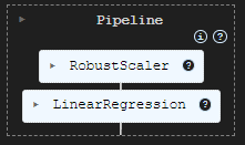
pipe_model = Pipeline([
    ("scaler", RobustScaler()),
    ("LR", LinearRegression())
])

pipe_model.fit(X_train, y_train) # Training a Linear regression model
输出
为了评估我们已有的模型,我决定基于训练和测试数据预测目标,将这些信息加入到一个 Pandas 数据帧,然后利用 Seaborn 和 Matplotlib 绘制成果。
# Preparing the data for plotting

train_pred = pipe_model.predict(X_train)
test_pred = pipe_model.predict(X_test)


train_data = pd.DataFrame({
    'Index': range(len(y_train)),
    'True Values': y_train,
    'Predicted Values': train_pred,
    'Set': 'Train'
})

test_data = pd.DataFrame({
    'Index': range(len(y_test)),
    'True Values': y_test,
    'Predicted Values': test_pred,
    'Set': 'Test'
})

# figure size 750x1000 pixels
fig, axes = plt.subplots(2, 1, figsize=(7.5, 10), sharex=False)

# Plot Train Data
sns.lineplot(ax=axes[0], data=train_data, x='Index', y='True Values', label='True Values', color='blue')
sns.lineplot(ax=axes[0], data=train_data, x='Index', y='Predicted Values', label='Predicted Values', color='orange')
axes[0].set_title(f'Train Set: True vs Predicted Values | Acc = {r2_score(y_train, train_pred)}', fontsize=14)
axes[0].set_ylabel('Values', fontsize=12)
axes[0].legend()

# Plot Test Data
sns.lineplot(ax=axes[1], data=test_data, x='Index', y='True Values', label='True Values', color='blue')
sns.lineplot(ax=axes[1], data=test_data, x='Index', y='Predicted Values', label='Predicted Values', color='orange')
axes[1].set_title(f'Test Set: True vs Predicted Values | Acc = {r2_score(y_test, test_pred)}', fontsize=14)
axes[1].set_xlabel('Index', fontsize=12)
axes[1].set_ylabel('Values', fontsize=12)
axes[1].legend()

# Final adjustments
plt.tight_layout()
plt.show()
输出
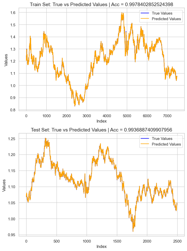
结果是一个约为 0.99 r2 分数的过拟合模型。这不是好的模型健康状况迹象。我们来审查特征的重要性,以便观察哪些特征对模型产生正面影响,而在检测到那些对模型有不良影响的特征时会被移除。
# Extract the linear regression model from the pipeline
lr_model = pipe_model.named_steps['LR']

# Get feature importance (coefficients)
feature_importance = pd.Series(lr_model.coef_, index=X_train.columns)

# Sort feature importance
feature_importance = feature_importance.sort_values(ascending=False)

print(feature_importance)
输出
macd main            266.706747
close                  0.093652
open                   0.093435
Avg price              0.042505
close lag_1            0.006972
close lag_3            0.003645
bb_upper               0.001423
close lag_5            0.001415
bb_middle              0.000766
high_low               0.000201
bb_lower               0.000087
var close 5 days      -0.000179
ATR 14                -0.000185
close pct_change      -0.001046
close lag_4           -0.002636
close lag_2           -0.003881
open_close            -0.004705
high                  -0.008575
low                   -0.008663
macd histogram     -5504.010453
macd signal        -5518.035201
dtype: float64
最具信息量的特征是 macd 主线,而 macd 直方图和 macd 信号则对模型来说信息量最少。我们舍弃掉所有负重要性的特征值,重新训练模型,然后再次观察准确率。
X = df.drop(columns=[
    "future_close", # drop the target veriable from the independent variables matrix
    "var close 5 days",
    "ATR 14",
    "close pct_change",
    "close lag_4",
    "close lag_2",
    "open_close",
    "high",
    "low",
    "macd histogram",
    "macd signal"
])
pipe_model = Pipeline([
    ("scaler", MinMaxScaler()),
    ("LR", LinearRegression())
])

pipe_model.fit(X_train, y_train)
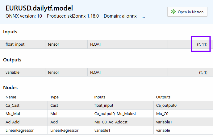
重新训练后的模型精度与之前的模型非常相似,但模型仍过拟合。对于目前这还好,接下来把模型导出到 ONNX 格式。
在 MQL5 中部署机器学习模型
在我们的智能系统(EA)中,我们首先将模型作为资源加载,以便与程序一起编译。
文件: LR model Test.mq5
#resource "\\Files\\EURUSD.dailytf.model.onnx" as uchar lr_onnx[]
我们导入了所有必要的函数库,包括 Pandas、ta-lib(用于指标)、和线性回归(用于加载模型)。
#include <Linear Regression.mqh>
#include <MALE5\pandas.mqh>
#include <ta-lib.mqh>

CLinearRegression lr;
我们在 OnInit 函数中初始化线性回归模型。
int OnInit()
  {
//---

   if (!lr.Init(lr_onnx))
     return INIT_FAILED;

//---
   return(INIT_SUCCEEDED);
  }
使用我们这个自定义的 Pandas 函数库的益处是,您不必从零开始写代码来重新收集数据,我们只需复制之前用过的代码,粘贴到智能系统之中,并做些微小修改。
void OnTick()
  {
//---

    CDataFrame df;
    int size = 10000; //We collect this amount of bars for training purposes

    vector open, high, low, close;
    open.CopyRates(Symbol(), PERIOD_D1, COPY_RATES_OPEN,1, size);
    high.CopyRates(Symbol(), PERIOD_D1, COPY_RATES_HIGH,1, size);
    low.CopyRates(Symbol(), PERIOD_D1, COPY_RATES_LOW,1, size);
    close.CopyRates(Symbol(), PERIOD_D1, COPY_RATES_CLOSE,1, size);

    df.Insert("open",open);
    df.Insert("high",high);
    df.Insert("low",low);
    df.Insert("close",close);


    int lags = 5;
    for (int i=1; i<=lags; i++)
      {
         vector lag = df.Shift("close", i);
         df.Insert("close lag_"+string(i), lag);
      }

    vector pct_change = df.Pct_change("close");
    df.Insert("close pct_change", pct_change);

    vector var_5 = df.Rolling("close", 5).Var();
    df.Insert("var close 5 days", var_5);

    df.Insert("open_close",open-close);
    df.Insert("high_low",high-low);

    df.Insert("Avg price",(open+high+low+close)/4);

//---

    BB_res_struct bb = CTrendIndicators::BollingerBands(close,20,0,2.000000); //Calculating the bollinger band indicator

    df.Insert("bb_lower",bb.lower_band); //Inserting lower band values
    df.Insert("bb_middle",bb.middle_band); //Inserting the middle band values
    df.Insert("bb_upper",bb.upper_band); //Inserting the upper band values

    vector atr = COscillatorIndicators::ATR(high,low,close,14);  //Calculating the ATR Indicator

    df.Insert("ATR 14",atr); //Inserting the ATR indicator values

    MACD_res_struct macd = COscillatorIndicators::MACD(close,12,26,9); //MACD indicator applied to the closing price

    df.Insert("macd histogram", macd.histogram); //Inserting the MAC historgram values
    df.Insert("macd main", macd.main); //Inserting the macd main line values
    df.Insert("macd signal", macd.signal);  //Inserting the macd signal line values

    df.Info();
    CDataFrame new_df = df.Dropnan();

    new_df.Head();

    string csv_name = Symbol()+".dailytf.data.csv";
    new_df.ToCSV(csv_name, false, 8);
  }
这些修改包括:
修改我们想要的数据大小。我们不再需要 10000 根柱线,只需要大约 30 根,因为 MACD 指标周期为 26,布林带周期为 20,ATR 周期为 14。将该值定为 30,我们实际上还预留了一些计算空间。
OnTick 函数有时流动性非常、且具爆发性,我们不需要每次接收到新即刻报价都重新定义变量。
我们不需要把数据保存到 CSV 文件里,只需把数据帧的最后一行赋值到一个向量当中,以便插入模型。
我们能把这些代码行打包成独立函数,从而工作起来更方便。
vector GetData(int start_bar=1, int size=30)
 {
    open_.CopyRates(Symbol(), PERIOD_D1, COPY_RATES_OPEN,start_bar, size);
    high_.CopyRates(Symbol(), PERIOD_D1, COPY_RATES_HIGH,start_bar, size);
    low_.CopyRates(Symbol(), PERIOD_D1, COPY_RATES_LOW,start_bar, size);
    close_.CopyRates(Symbol(), PERIOD_D1, COPY_RATES_CLOSE,start_bar, size);

    df_.Insert("open",open_);
    df_.Insert("high",high_);
    df_.Insert("low",low_);
    df_.Insert("close",close_);


    int lags = 5;
    vector lag = {};

    for (int i=1; i<=lags; i++)
      {
         lag = df_.Shift("close", i);
         df_.Insert("close lag_"+string(i), lag);
      }

    pct_change = df_.Pct_change("close");
    df_.Insert("close pct_change", pct_change);

    var_5 = df_.Rolling("close", 5).Var();
    df_.Insert("var close 5 days", var_5);

    df_.Insert("open_close",open_-close_);
    df_.Insert("high_low",high_-low_);

    df_.Insert("Avg price",(open_+high_+low_+close_)/4);

//---

    BB_res_struct bb = CTrendIndicators::BollingerBands(close_,20,0,2.000000); //Calculating the bollinger band indicator

    df_.Insert("bb_lower",bb.lower_band); //Inserting lower band values
    df_.Insert("bb_middle",bb.middle_band); //Inserting the middle band values
    df_.Insert("bb_upper",bb.upper_band); //Inserting the upper band values

    atr = COscillatorIndicators::ATR(high_,low_,close_,14);  //Calculating the ATR Indicator

    df_.Insert("ATR 14",atr); //Inserting the ATR indicator values

    MACD_res_struct macd = COscillatorIndicators::MACD(close_,12,26,9); //MACD indicator applied to the closing price

    df_.Insert("macd histogram", macd.histogram); //Inserting the MAC historgram values
    df_.Insert("macd main", macd.main); //Inserting the macd main line values
    df_.Insert("macd signal", macd.signal);  //Inserting the macd signal line values


    CDataFrame new_df = df_.Dropnan(); //Drop NaN values
    return new_df.Loc(-1); //return the latest row
 }
这就是我们如何初步收集训练数据的方式,函数中的一些特征由于各种原因未能进入最终模型,我们不得不放弃它们,就像我们在 Python 脚本中删除它们一样。
vector GetData(int start_bar=1, int size=30)
 {
    open_.CopyRates(Symbol(), PERIOD_D1, COPY_RATES_OPEN,start_bar, size);
    high_.CopyRates(Symbol(), PERIOD_D1, COPY_RATES_HIGH,start_bar, size);
    low_.CopyRates(Symbol(), PERIOD_D1, COPY_RATES_LOW,start_bar, size);
    close_.CopyRates(Symbol(), PERIOD_D1, COPY_RATES_CLOSE,start_bar, size);

    df_.Insert("open",open_);
    df_.Insert("high",high_);
    df_.Insert("low",low_);
    df_.Insert("close",close_);


    int lags = 5;
    vector lag = {};

    for (int i=1; i<=lags; i++)
      {
         lag = df_.Shift("close", i);
         df_.Insert("close lag_"+string(i), lag);
      }

    pct_change = df_.Pct_change("close");
    df_.Insert("close pct_change", pct_change);

    var_5 = df_.Rolling("close", 5).Var();
    df_.Insert("var close 5 days", var_5);

    df_.Insert("open_close",open_-close_);
    df_.Insert("high_low",high_-low_);

    df_.Insert("Avg price",(open_+high_+low_+close_)/4);

//---

    BB_res_struct bb = CTrendIndicators::BollingerBands(close_,20,0,2.000000); //Calculating the bollinger band indicator

    df_.Insert("bb_lower",bb.lower_band); //Inserting lower band values
    df_.Insert("bb_middle",bb.middle_band); //Inserting the middle band values
    df_.Insert("bb_upper",bb.upper_band); //Inserting the upper band values

    atr = COscillatorIndicators::ATR(high_,low_,close_,14);  //Calculating the ATR Indicator

    df_.Insert("ATR 14",atr); //Inserting the ATR indicator values

    MACD_res_struct macd = COscillatorIndicators::MACD(close_,12,26,9); //MACD indicator applied to the closing price

    df_.Insert("macd histogram", macd.histogram); //Inserting the MAC historgram values
    df_.Insert("macd main", macd.main); //Inserting the macd main line values
    df_.Insert("macd signal", macd.signal);  //Inserting the macd signal line values


    df_ = df_.Drop(
       //"future_close",
       "var close 5 days,"+
       "ATR 14,"+
       "close pct_change,"+
       "close lag_4,"+
       "close lag_2,"+
       "open_close,"+
       "high,"+
       "low,"+
       "macd histogram,"+
       "macd signal"
    );

    CDataFrame new_df = df_.Dropnan();

    return new_df.Loc(-1); //return the latest row
 }
与上述函数中舍弃列不同, 明智的做法是删除最初用于生成这些特征的代码,这样可以减少不必要的计算,避免程序变慢,因为需要计算的特征很多,它们很快便被舍弃。
我们暂时会坚持使用 Drop 方法。
调用 Head() 方法查看数据帧上的内容之后,结果如下:
PM      0       15:45:36.543    LR model Test (EURUSD,H1)       CDataFrame::Dropnan completed. Rows dropped: 25/30
HI      0       15:45:36.543    LR model Test (EURUSD,H1)       | open           | close          | close lag_1     | close lag_3     | close lag_5     | high_low       | Avg price      | bb_lower       | bb_middle      | bb_upper       | macd main      |
GK      0       15:45:36.543    LR model Test (EURUSD,H1)       | 1.04057000     | 1.04079000     | 1.04057000      | 1.02806000      | 1.03015000      | 0.00575000     | 1.04176750     | 1.02125891     | 1.03177350     | 1.04228809     | 0.00028705     |
QI      0       15:45:36.543    LR model Test (EURUSD,H1)       | 1.04079000     | 1.04159000     | 1.04079000      | 1.04211000      | 1.02696000      | 0.00661000     | 1.04084750     | 1.02081967     | 1.03210400     | 1.04338833     | 0.00085370     |
PL      0       15:45:36.543    LR model Test (EURUSD,H1)       | 1.04158000     | 1.04956000     | 1.04159000      | 1.04057000      | 1.02806000      | 0.01099000     | 1.04611250     | 1.01924805     | 1.03282750     | 1.04640695     | 0.00192371     |
JR      0       15:45:36.543    LR model Test (EURUSD,H1)       | 1.04795000     | 1.04675000     | 1.04956000      | 1.04079000      | 1.04211000      | 0.00204000     | 1.04743000     | 1.01927184     | 1.03382650     | 1.04838116     | 0.00251595     |
CP      0       15:45:36.543    LR model Test (EURUSD,H1)       | 1.04675000     | 1.04370000     | 1.04675000      | 1.04159000      | 1.04057000      | 0.01049000     | 1.04664500     | 1.01938012     | 1.03447300     | 1.04956588     | 0.00270798     |
CH      0       15:45:36.543    LR model Test (EURUSD,H1)       (5x11)
我们有 11 个特征,模型上能够看到同样数量的特征。
以下是我们如何获得最终模型的预测。
void OnTick()
  {
     vector x = GetData();
     Comment("Predicted close: ", lr.predict(x));
  }
不应该在每次即刻报价都做一遍所有数据收集和模型计算,我们只需在图表新柱线开立时计算。
void OnTick()
  {
     if (isNewBar())
       {
           vector x = GetData();
           Comment("Predicted close: ", lr.predict(x));
       }
  }
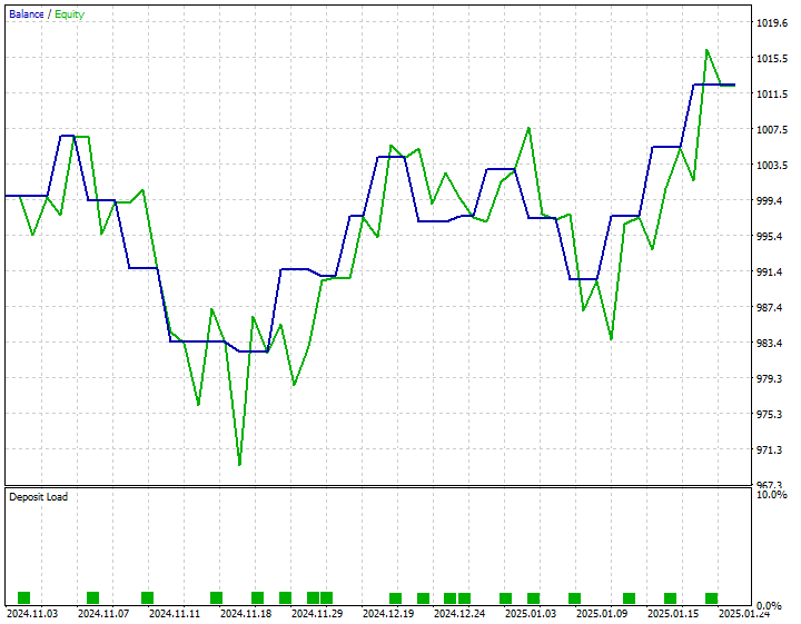
我开发了一个简单的策略:当预测收盘价高于当前出价时下单买入交易,当预测收盘价低于当前要价时下单卖出交易。
以下是 2024 年 11 月 1 日至 2025 年 1 月 25 日的策略测试结果。
结束语
现在将复杂的 AI 模型导入 MQL5,并在 MetaTrader 5 使用它们已很轻松,但保持模型与训练数据结构的同步仍然不容易。在本文中,我讲述了一个名为 CDataframe 的自定义类,帮助我们在处理二维数据时,类似 Pandas 函数库中环境中所用,而 Pandas 函数库对机器学习社区,和来自 Python 背景的数据科学家来说非常熟悉。
我希望 MQL5 中的 Pandas 函数库能发挥作用,令我们在处理复杂 AI 数据时更加轻松。
此致敬意。
敬请关注,并在这个 GitHub 仓储库中为 MQL5 语言的机器学习算法开发做出贡献。
附件表
| 文件名 | 说明/用法 |
|---|---|
| Experts\LR model Test.mq5 | 一款智能系统,用于部署最终线性回归模型。 |
| Include\Linear Regression.mqh | 一个包含所有加载 ONNX 格式线性回归模型的代码库。 |
| Include\pandas.mqh | 包含所有处理 Dataframe 类数据的 Pandas 自定义方法。 |
| Scripts\pandas test.mq5 | 一个负责收集机器学习训练数据的脚本。 |
| Python\main.ipynb | 一个 Jupyter 笔记簿文件,包含本文中用到的所有线性回归模型训练代码。 |
| 文件 | 该文件夹包含 ONNX 模型中的线性回归模型,和 AI 模型训练的 CSV 文件。 |
本文由MetaQuotes Ltd译自英文
原文地址: https://www.mql5.com/en/articles/17030
注意: MetaQuotes Ltd.将保留所有关于这些材料的权利。全部或部分复制或者转载这些材料将被禁止。
本文由网站的一位用户撰写,反映了他们的个人观点。MetaQuotes Ltd 不对所提供信息的准确性负责,也不对因使用所述解决方案、策略或建议而产生的任何后果负责。
