
如何在 MQL5 中使用 ONNX 模型

概述
文章《基于CNN-LSTM的股票价格预测模型》(卢文杰、李佳正、李一凡、孙爱军、王景阳(所有姓名音译),《复杂性》杂志, 2020 年卷,文章 ID 6622927,10 页,2020)的作者比较了各种股价预测模型:
股价数据具有时间序列的特征。
与此同时,基于机器学习长短期记忆(LSTM),通过其记忆函数分析时间序列数据之间的关系,提出一种基于 CNN-LSTM 的股价预测方法。
同时,我们使用 MLP、CNN、RNN、LSTM、CNN-RNN,等预测模型逐一预测股价。 甚而,还对这些模型的预测结果进行了分析和比较。 本项研究中使用的数据取自 1991 年 7 月 31 日至 2020 年 8 月 31 日的日线股票价格,包括 7127 个交易日。
在历史数据方面,我们选择八个特征,包括开盘价、最高价、最低价、收盘价、成交量、成交量、涨跌幅和变化。
首先,我们采用 CNN 从数据中有效地提取特征,即前 10 天的数据项。 然后,我们采用 LSTM 利用提取的特征数据预测股价。
根据实验结果,CNN-LSTM 可以提供可靠的,具有最高预测精度的股价预测。
这种预测方法不仅为股价预测提供了新的研究思路,也为学者研究金融时间序列数据提供了实践经验。
在所有研究的模型中,CNN-LSTM 模型在实验过程中产生了最好的结果。 在本文中,我们将研究如何创建这样的模型来预测金融时间序列,以及如何在 MQL5 智能系中运用创建的 ONNX 模型。
1. 构建模型
Python 提供了一组专门的函数库,因此它提供了处理机器学习模型的广泛功能。 函数库极大地方便了数据的准备和处理。
我们建议使用 GPU 资源来最大限度地提高机器学习项目的效率。 许多 Windows 用户在尝试安装当前的 TensorFlow 版本时遇到了问题(请参阅视频指南,及其文本版本的注释)。 故此,我们已经测试了TensorFlow 2.10.0,并建议使用此版本。 GPU 计算是在 NVIDIA GeForce RTX 2080 Ti 图形卡上使用 CUDA 11.2 和 CUDNN 8.1.0.7 函数库进行的。
1.1. 安装 Python 和函数库
如果您还没有 Python,请您先安装它。 我们使用的是 3.9.16 版。
另外,还要安装函数库(如果您使用的是 Conda/Anaconda,请在 Anaconda 提示符下运行以下命令):
python.exe -m pip install --upgrade pip
pip install --upgrade pandas
pip install --upgrade scikit-learn
pip install --upgrade matplotlib
pip install --upgrade tqdm
pip install --upgrade metatrader5
pip install --upgrade onnx==1.12
pip install --upgrade tf2onnx
pip install --upgrade tensorflow==2.10.0
1.2. 检查 TensorFlow 版本和 GPU
下面的代码检查已安装的 TensorFlow 版本,并验证是否可以使用 GPU 来计算模型:
#check tensorflow version
print(tf.__version__)
#check GPU support
print(len(tf.config.list_physical_devices('GPU'))>0)
如果正确安装了所需的版本,您将看到以下结果:
True
我们使用 Python 脚本来构建和训练模型。 下面简要介绍此过程的步骤。
1.3. 构建和训练模型
该脚本首先导入将在模型中使用的 Python 函数库。
#Python libraries
import matplotlib.pyplot as plt
import MetaTrader5 as mt5
import tensorflow as tf
import numpy as np
import pandas as pd
import tf2onnx
from sklearn.model_selection import train_test_split
from sys import argv
检查 TensorFlow 版本和 GPU 可用性:
#check tensorflow version
print(tf.__version__)
2.10.0
#check GPU support
print(len(tf.config.list_physical_devices('GPU'))>0)
True
初始化 MetaTrader 5 以执行来自 Python 的操作:
#initialize MetaTrader5 for history data
if not mt5.initialize():
    print("initialize() failed, error code =",mt5.last_error())
    quit()
有关 MetaTrader 5 终端的信息:
#show terminal info
terminal_info=mt5.terminal_info()
print(terminal_info)
TerminalInfo(community_account=True, community_connection=True, connected=True, dlls_allowed=False, trade_allowed=False, tradeapi_disabled=False, email_enabled=False, ftp_enabled=False, notifications_enabled=False, mqid=False, build=3640, maxbars=100000, codepage=0, ping_last=58768, community_balance=1.0, retransmission=0.015296317559440137, company='MetaQuotes Software Corp.', name='MetaTrader 5', language='English', path='C:\\Program Files\\MetaTrader 5', data_path='C:\\Users\\user\\AppData\\Roaming\\MetaQuotes\\Terminal\\D0E8209F77C8CF37AD8BF550E51FF075', commondata_path='C:\\Users\\user\\AppData\\Roaming\\MetaQuotes\\Terminal\\Common')
#show file path
file_path=terminal_info.data_path+"\\MQL5\\Files\\"
print(file_path)
打印模型(在此示例中,脚本在 Jupyter 笔记本中运行)的保存路径:
#data path to save the model
data_path=argv[0]
last_index=data_path.rfind("\\")+1
data_path=data_path[0:last_index]
print("data path to save onnx model",data_path)
data path to save onnx model C:\Users\user\AppData\Roaming\Python\Python39\site-packages\
准备请求历史数据的日期。 在我们的示例中,我们请求从当前日期开始 120 根 EURUSD H1 的柱线:
#set start and end dates for history data
from datetime import timedelta,datetime
end_date = datetime.now()
start_date = end_date - timedelta(days=120)

#print start and end dates
print("data start date=",start_date)
print("data end date=",end_date)
data end date= 2023-03-28 12:28:39.870685
请求 EURUSD 历史数据:
#get EURUSD rates (H1) from start_date to end_date
eurusd_rates = mt5.copy_rates_range("EURUSD", mt5.TIMEFRAME_H1, start_date, end_date)
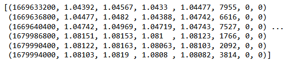
输出下载的数据:
#check
print(eurusd_rates)
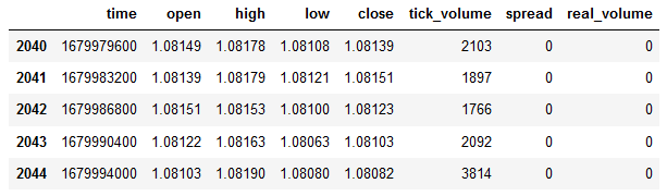
#create dataframe
df = pd.DataFrame(eurusd_rates)
显示数据帧的开始和结束:
#show dataframe head
df.head()

#show dataframe tail
df.tail()
#show dataframe shape (the number of rows and columns in the data set)
df.shape
(2045, 8)
仅选择收盘价:
#prepare close prices only
data = df.filter(['close']).values
输出数据:
#show close prices
plt.figure(figsize = (18,10))
plt.plot(data,'b',label = 'Original')
plt.xlabel("Hours")
plt.ylabel("Price")
plt.title("EURUSD_H1")
plt.legend()

使用 MinMaxScaler 将源价格数据缩放到范围 [0,1]:
#scale data using MinMaxScaler
from sklearn.preprocessing import MinMaxScaler
scaler=MinMaxScaler(feature_range=(0,1))
scaled_data = scaler.fit_transform(data)
前 80% 的数据将用于训练。
#training size is 80% of the data
training_size = int(len(scaled_data)*0.80)
print("training size:",training_size)
training size: 1636
#create train data and check size
train_data_initial = scaled_data[0:training_size,:]
print(len(train_data_initial))
1636
#create test data and check size
test_data_initial= scaled_data[training_size:,:1]
print(len(test_data_initial))
409
以下函数创建训练序列:
#split a univariate sequence into samples
def split_sequence(sequence, n_steps):
    X, y = list(), list()
    for i in range(len(sequence)):
       #find the end of this pattern
       end_ix = i + n_steps
       #check if we are beyond the sequence
       if end_ix > len(sequence)-1:
          break
       #gather input and output parts of the pattern
       seq_x, seq_y = sequence[i:end_ix], sequence[end_ix]
       X.append(seq_x)
       y.append(seq_y)
    return np.array(X), np.array(y)
构建集合:
#split into samples
time_step = 120
x_train, y_train = split_sequence(train_data_initial, time_step)
x_test, y_test = split_sequence(test_data_initial, time_step)
#reshape input to be [samples, time steps, features] which is required for LSTM
x_train =x_train.reshape(x_train.shape[0],x_train.shape[1],1)
x_test = x_test.reshape(x_test.shape[0],x_test.shape[1],1)
用于训练和测试的张量形状:
#show shape of train data
x_train.shape
(1516, 120, 1)
#show shape of test data
x_test.shape
(289, 120, 1)
#import keras libraries for the model
import math
from keras.models import Sequential
from keras.layers import Dense,Activation,Conv1D,MaxPooling1D,Dropout
from keras.layers import LSTM
from keras.utils.vis_utils import plot_model
from keras.metrics import RootMeanSquaredError as rmse
from keras import optimizers
设置模型:
#define the model
model = Sequential()
model.add(Conv1D(filters=256, kernel_size=2,activation='relu',padding = 'same',input_shape=(120,1)))
model.add(MaxPooling1D(pool_size=2))
model.add(LSTM(100, return_sequences = True))
model.add(Dropout(0.3))
model.add(LSTM(100, return_sequences = False))
model.add(Dropout(0.3))
model.add(Dense(units=1, activation = 'sigmoid'))
model.compile(optimizer='adam', loss= 'mse' , metrics = [rmse()])
显示模型属性:
#show model
model.summary()

模型训练:
#measure time
import time
time_calc_start = time.time()

#fit model with 300 epochs
history=model.fit(x_train,y_train,epochs=300,validation_data=(x_test,y_test),batch_size=32,verbose=1)

#calculate time
fit_time_seconds = time.time() - time_calc_start
print("fit time =",fit_time_seconds," seconds.")
Epoch 1/300
48/48 [==============================] - 8s 49ms/step - loss: 0.0129 - root_mean_squared_error: 0.1136 - val_loss: 0.0065 - val_root_mean_squared_error: 0.0804
...
Epoch 299/300
48/48 [==============================] - 2s 35ms/step - loss: 4.5197e-04 - root_mean_squared_error: 0.0213 - val_loss: 4.2535e-04 - val_root_mean_squared_error: 0.0206
Epoch 300/300
48/48 [==============================] - 2s 32ms/step - loss: 4.2967e-04 - root_mean_squared_error: 0.0207 - val_loss: 4.4040e-04 - val_root_mean_squared_error: 0.0210
fit time = 467.4918096065521 seconds.
训练大约需要 8 分钟。
#show training history keys
history.history.keys()
训练和测试数据集中的优化动态:
#show iteration-loss graph for training and validation
plt.figure(figsize = (18,10))
plt.plot(history.history['loss'],label='Training Loss',color='b')
plt.plot(history.history['val_loss'],label='Validation-loss',color='g')
plt.xlabel("Iteration")
plt.ylabel("Loss")
plt.title("LOSS")
plt.legend()

#show iteration-rmse graph for training and validation
plt.figure(figsize = (18,10))
plt.plot(history.history['root_mean_squared_error'],label='Training RMSE',color='b')
plt.plot(history.history['val_root_mean_squared_error'],label='Validation-RMSE',color='g')
plt.xlabel("Iteration")
plt.ylabel("RMSE")
plt.title("RMSE")
plt.legend()

#evaluate training data
model.evaluate(x_train,y_train, batch_size = 32)
[0.00029911252204328775, 0.01729486882686615]
#evaluate testing data
model.evaluate(x_test,y_test, batch_size = 32)
10/10 [==============================] - 0s 31ms/step - loss: 4.4040e-04 - root_mean_squared_error: 0.0210
[0.00044039846397936344, 0.020985672250390053]
依据训练数据集形成预测:
#prediction using training data
train_predict = model.predict(x_train)
plot_y_train = y_train.reshape(-1,1)
输出训练间隔的实际和预测图形:
#show actual vs predicted (training) graph
plt.figure(figsize=(18,10))
plt.plot(scaler.inverse_transform(plot_y_train),color = 'b', label = 'Original')
plt.plot(scaler.inverse_transform(train_predict),color='red', label = 'Predicted')
plt.title("Prediction Graph Using Training Data")
plt.xlabel("Hours")
plt.ylabel("Price")
plt.legend()
plt.show()

依据测试数据集形成预测:
#prediction using testing data
test_predict = model.predict(x_test)
plot_y_test = y_test.reshape(-1,1)
11/11 [==============================] - 0s 11ms/step
为了计算指标,我们需要转换区间 [0,1] 中的数据。 同样,我们使用 MinMaxScaler。
#calculate metrics
from sklearn import metrics
from sklearn.metrics import r2_score
#transform data to real values
value1=scaler.inverse_transform(plot_y_test)
value2=scaler.inverse_transform(test_predict)
#calc score
score = np.sqrt(metrics.mean_squared_error(value1,value2))
print("RMSE         : {}".format(score))
print("MSE          :", metrics.mean_squared_error(value1,value2))
print("R2 score     :",metrics.r2_score(value1,value2))
RMSE : 0.0015151631684117558
MSE : 2.295719426911551e-06
R2 score : 0.9683533377809039
#show actual vs predicted (testing) graph
plt.figure(figsize=(18,10))
plt.plot(scaler.inverse_transform(plot_y_test),color = 'b',  label = 'Original')
plt.plot(scaler.inverse_transform(test_predict),color='g', label = 'Predicted')
plt.title("Prediction Graph Using Testing Data")
plt.xlabel("Hours")
plt.ylabel("Price")
plt.legend()
plt.show()

将模型导出到 onnx 文件:
# save model to ONNX
output_path = data_path+"model.eurusd.H1.120.onnx"
onnx_model = tf2onnx.convert.from_keras(model, output_path=output_path)
print(f"model saved to {output_path}")

output_path = file_path+"model.eurusd.H1.120.onnx"
onnx_model = tf2onnx.convert.from_keras(model, output_path=output_path)
print(f"saved model to {output_path}")

# finish
mt5.shutdown()
Python 脚本的完整代码附于 Jupyter Notebook 文章的文后。
在文章基于 CNN-LSTM 的股票价格预测模型中,针对具有 CNN-LSTM 架构的模型,获得了最佳结果 R^2=0.9646。 在我们的示例中,CNN-LSTM 网络生成了 R^2=0.9684 的最佳结果。 根据结果,这种类型的模型可以有效地解决预测问题。
我们已研究了一个 Python 脚本的例子,它构建和训练 CNN-LSTM 模型来预测金融时间序列。
2. 在 MT5 中运用模型
2.1. 在开始之前最好知道
有两种途径可以创建模型:可以使用 OnnxCreate 从 onnx 文件创建模型;亦或使用 OnnxCreateFromBuffer 从数据数组创建模型。
如果将 ONNX 模型用作 EA 中的资源,则每次更改模型时都需要重新编译 EA。
并非所有模型都有完全定义的输入和/或输出张量大小。 正常情况下,第一个维度负责封包大小。 在运行模型之前,必须使用 OnnxSetInputShape 和 OnnxSetOutputShape 函数显式指定大小。 模型的输入数据理应与训练模型时的准备方式相同。
对于输入和输出数据,我们建议使用模型中使用的相同类型的数组、矩阵和/或向量。 在这种情况下,运行模型时不必进行数据转换。 如果数据无法以所需类型表示,则数据将自动转换。
您的模型需调用 OnnxRun 函数来推断(运行)。 请注意,一个模型可以运行多次。 模型使用完毕,调用 OnnxRelease 函数释放它。
2.2. 读取 onnx 文件,并获取有关输入和输出的信息
为了使用我们的模型,我们需要知道模型位置、输入数据类型和形状,以及输出数据类型和形状。 根据之前创建的脚本,model.eurusd.H1.120.onnx 与生成 onnx 文件的 Python 脚本位于相同的文件夹之中。 输入为 float32,120 个常规化收盘价(适用于批次大小等于 1);输出为 float32,这是模型预测的一个常规化价格。
我们还在 MQL5\Files 文件夹中创建了 onnx 文件,以便利用 MQL5 脚本获取模型输入和输出数据。
//+------------------------------------------------------------------+
//|                                                OnnxModelInfo.mq5 |
//|                                  Copyright 2023, MetaQuotes Ltd. |
//|                                             https://www.mql5.com |
//+------------------------------------------------------------------+
#property copyright "Copyright 2023, MetaQuotes Ltd."
#property link      "https://www.mql5.com"
#property version   "1.00"

#define UNDEFINED_REPLACE 1

//+------------------------------------------------------------------+
//| Script program start function                                    |
//+------------------------------------------------------------------+
void OnStart()
  {
   string file_names[];
   if(FileSelectDialog("Open ONNX model",NULL,"ONNX files (*.onnx)|*.onnx|All files (*.*)|*.*",FSD_FILE_MUST_EXIST,file_names,NULL)<1)
      return;

   PrintFormat("Create model from %s with debug logs",file_names[0]);

   long session_handle=OnnxCreate(file_names[0],ONNX_DEBUG_LOGS);
   if(session_handle==INVALID_HANDLE)
     {
      Print("OnnxCreate error ",GetLastError());
      return;
     }

   OnnxTypeInfo type_info;

   long input_count=OnnxGetInputCount(session_handle);
   Print("model has ",input_count," input(s)");
   for(long i=0; i<input_count; i++)
     {
      string input_name=OnnxGetInputName(session_handle,i);
      Print(i," input name is ",input_name);
      if(OnnxGetInputTypeInfo(session_handle,i,type_info))
         PrintTypeInfo(i,"input",type_info);
     }

   long output_count=OnnxGetOutputCount(session_handle);
   Print("model has ",output_count," output(s)");
   for(long i=0; i<output_count; i++)
     {
      string output_name=OnnxGetOutputName(session_handle,i);
      Print(i," output name is ",output_name);
      if(OnnxGetOutputTypeInfo(session_handle,i,type_info))
         PrintTypeInfo(i,"output",type_info);
     }

   OnnxRelease(session_handle);
  }
//+------------------------------------------------------------------+
//| PrintTypeInfo                                                    |
//+------------------------------------------------------------------+
void PrintTypeInfo(const long num,const string layer,const OnnxTypeInfo& type_info)
  {
   Print("   type ",EnumToString(type_info.type));
   Print("   data type ",EnumToString(type_info.element_type));

   if(type_info.dimensions.Size()>0)
     {
      bool   dim_defined=(type_info.dimensions[0]>0);
      string dimensions=IntegerToString(type_info.dimensions[0]);
      for(long n=1; n<type_info.dimensions.Size(); n++)
        {
         if(type_info.dimensions[n]<=0)
            dim_defined=false;
         dimensions+=", ";
         dimensions+=IntegerToString(type_info.dimensions[n]);
        }
      Print("   shape [",dimensions,"]");
      //--- not all dimensions defined
      if(!dim_defined)
         PrintFormat("   %I64d %s shape must be defined explicitly before model inference",num,layer);
      //--- reduce shape
      uint reduced=0;
      long dims[];
      for(long n=0; n<type_info.dimensions.Size(); n++)
        {
         long dimension=type_info.dimensions[n];
         //--- replace undefined dimension
         if(dimension<=0)
            dimension=UNDEFINED_REPLACE;
         //--- 1 can be reduced
         if(dimension>1)
           {
            ArrayResize(dims,reduced+1);
            dims[reduced++]=dimension;
           }
        }
      //--- all dimensions assumed 1
      if(reduced==0)
        {
         ArrayResize(dims,1);
         dims[reduced++]=1;
        }
      //--- shape was reduced
      if(reduced<type_info.dimensions.Size())
        {
         dimensions=IntegerToString(dims[0]);
         for(long n=1; n<dims.Size(); n++)
           {
            dimensions+=", ";
            dimensions+=IntegerToString(dims[n]);
           }
         string sentence="";
         if(!dim_defined)
            sentence=" if undefined dimension set to "+(string)UNDEFINED_REPLACE;
         PrintFormat("   shape of %s data can be reduced to [%s]%s",layer,dimensions,sentence);
        }
     }
   else
      PrintFormat("no dimensions defined for %I64d %s",num,layer);
  }
//+------------------------------------------------------------------+
在文件选择窗口中,我们选择了保存在 MQL5\Files 中的 onnx 文件,调用 OnnxCreate 从该文件创建了一个模型,并获得了以下信息。
Create model from model.eurusd.H1.120.onnx with debug logs
ONNX: Creating and using per session threadpools since use_per_session_threads_ is true
ONNX: Dynamic block base set to 0
ONNX: Initializing session.
ONNX: Adding default CPU execution provider.
ONNX: Total shared scalar initializer count: 0
ONNX: Total fused reshape node count: 0
ONNX: Removing NodeArg 'Gather_out0'. It is no longer used by any node.
ONNX: Removing NodeArg 'Gather_token_1_out0'. It is no longer used by any node.
ONNX: Total shared scalar initializer count: 0
ONNX: Total fused reshape node count: 0
ONNX: Removing initializer 'sequential/conv1d/Conv1D/ExpandDims_1:0'. It is no longer used by any node.
ONNX: Use DeviceBasedPartition as default
ONNX: Saving initialized tensors.
ONNX: Done saving initialized tensors
ONNX: Session successfully initialized.
model has 1 input(s)
0 input name is conv1d_input
   type ONNX_TYPE_TENSOR
   data type ONNX_DATA_TYPE_FLOAT
   shape [-1, 120, 1]
   0 input shape must be defined explicitly before model inference
   shape of input data can be reduced to [120] if undefined dimension set to 1
model has 1 output(s)
0 output name is dense
   type ONNX_TYPE_TENSOR
   data type ONNX_DATA_TYPE_FLOAT
   shape [-1, 1]
   0 output shape must be defined explicitly before model inference
   shape of output data can be reduced to [1] if undefined dimension set to 1
由于启用了调试模式
long session_handle=OnnxCreate(file_names[0],ONNX_DEBUG_LOGS);
我们有带有 ONNX 前缀的日志。
我们看到模型实际上有一个输入和一个输出。 此处,输入张量的第一维和输出张量的第一维没有定义。 假定这些维度负责批次大小。 因此,在推断模型之前,我们必须明确指定我们将要使用的大小(OnnxSetInputShape 和 OnnxSetOutputShape)。 通常只有一个数据集会被输入到模型中。 下一段“在交易 EA 中使用 ONNX 模型的示例”中提供了一个详细示例。
准备数据时,不必使用维度为 [1, 120, 1] 的数组。 我们可以输入一维数组或一个 120 个元素的向量。
2.3. 在交易 EA 中使用 ONNX 模型的示例
声明和定义
#include <Trade\Trade.mqh>

input double InpLots = 1.0;    // Lots amount to open position

#resource "Python/model.120.H1.onnx" as uchar ExtModel[]

#define SAMPLE_SIZE 120

long     ExtHandle=INVALID_HANDLE;
int      ExtPredictedClass=-1;
datetime ExtNextBar=0;
datetime ExtNextDay=0;
float    ExtMin=0.0;
float    ExtMax=0.0;
CTrade   ExtTrade;

//--- price movement prediction
#define PRICE_UP   0
#define PRICE_SAME 1
#define PRICE_DOWN 2
OnInit 函数
//+------------------------------------------------------------------+
//| Expert initialization function                                   |
//+------------------------------------------------------------------+
int OnInit()
  {
   if(_Symbol!="EURUSD" || _Period!=PERIOD_H1)
     {
      Print("model must work with EURUSD,H1");
      return(INIT_FAILED);
     }

//--- create a model from static buffer
   ExtHandle=OnnxCreateFromBuffer(ExtModel,ONNX_DEFAULT);
   if(ExtHandle==INVALID_HANDLE)
     {
      Print("OnnxCreateFromBuffer error ",GetLastError());
      return(INIT_FAILED);
     }

//--- since not all sizes defined in the input tensor we must set them explicitly
//--- first index - batch size, second index - series size, third index - number of series (only Close)
   const long input_shape[] = {1,SAMPLE_SIZE,1};
   if(!OnnxSetInputShape(ExtHandle,ONNX_DEFAULT,input_shape))
     {
      Print("OnnxSetInputShape error ",GetLastError());
      return(INIT_FAILED);
     }

//--- since not all sizes defined in the output tensor we must set them explicitly
//--- first index - batch size, must match the batch size of the input tensor
//--- second index - number of predicted prices (we only predict Close)
   const long output_shape[] = {1,1};
   if(!OnnxSetOutputShape(ExtHandle,0,output_shape))
     {
      Print("OnnxSetOutputShape error ",GetLastError());
      return(INIT_FAILED);
     }
//---
   return(INIT_SUCCEEDED);
  }
我们只处理 EURUSD, H1,因为我们使用当前的交易品种/周期数据。
我们的模型作为资源包含在 EA 之中。 EA 是完全自给自足的,不需要读取外部 onnx 文件。 从资源数组创建模型。
必须显式定义输入和输出数据形状。
OnTick 函数:
//+------------------------------------------------------------------+
//| Expert tick function                                             |
//+------------------------------------------------------------------+
void OnTick()
  {
//--- check new day
   if(TimeCurrent()>=ExtNextDay)
     {
      GetMinMax();
      //--- set next day time
      ExtNextDay=TimeCurrent();
      ExtNextDay-=ExtNextDay%PeriodSeconds(PERIOD_D1);
      ExtNextDay+=PeriodSeconds(PERIOD_D1);
     }

//--- check new bar
   if(TimeCurrent()<ExtNextBar)
      return;
//--- set next bar time
   ExtNextBar=TimeCurrent();
   ExtNextBar-=ExtNextBar%PeriodSeconds();
   ExtNextBar+=PeriodSeconds();
//--- check min and max
   double close=iClose(_Symbol,_Period,0);
   if(ExtMin>close)
      ExtMin=close;
   if(ExtMax<close)
      ExtMax=close;

//--- predict next price
   PredictPrice();
//--- check trading according to prediction
   if(ExtPredictedClass>=0)
      if(PositionSelect(_Symbol))
         CheckForClose();
      else
         CheckForOpen();
  }
我们定义新一天的开始。 从日期开始用于更新 120 天序列的“最低价”和“最高价”的数值,从而常规化 120 小时序列中的价格。 模型是在这些条件下训练的,我们在准备输入数据时必须遵循这些条件。
//+------------------------------------------------------------------+
//| Get minimal and maximal Close for last 120 days                  |
//+------------------------------------------------------------------+
void GetMinMax(void)
  {
   vectorf close;
   close.CopyRates(_Symbol,PERIOD_D1,COPY_RATES_CLOSE,0,SAMPLE_SIZE);
   ExtMin=close.Min();
   ExtMax=close.Max();
  }
如有必要,我们可以修改全天的最低价和最高价。
预测函数:
//+------------------------------------------------------------------+
//| Predict next price                                               |
//+------------------------------------------------------------------+
void PredictPrice(void)
  {
   static vectorf output_data(1);            // vector to get result
   static vectorf x_norm(SAMPLE_SIZE);       // vector for prices normalize

//--- check for normalization possibility
   if(ExtMin>=ExtMax)
     {
      ExtPredictedClass=-1;
      return;
     }
//--- request last bars
   if(!x_norm.CopyRates(_Symbol,_Period,COPY_RATES_CLOSE,1,SAMPLE_SIZE))
     {
      ExtPredictedClass=-1;
      return;
     }
   float last_close=x_norm[SAMPLE_SIZE-1];
//--- normalize prices
   x_norm-=ExtMin;
   x_norm/=(ExtMax-ExtMin);
//--- run the inference
   if(!OnnxRun(ExtHandle,ONNX_NO_CONVERSION,x_norm,output_data))
     {
      ExtPredictedClass=-1;
      return;
     }
//--- denormalize the price from the output value
   float predicted=output_data[0]*(ExtMax-ExtMin)+ExtMin;
//--- classify predicted price movement
   float delta=last_close-predicted;
   if(fabs(delta)<=0.00001)
      ExtPredictedClass=PRICE_SAME;
   else
     {
      if(delta<0)
         ExtPredictedClass=PRICE_UP;
      else
         ExtPredictedClass=PRICE_DOWN;
     }
  }
首先,我们检查是否可以常规化。 常规化的实现如同 MinMaxScaler Python 函数。
#scale data
from sklearn.preprocessing import MinMaxScaler
scaler=MinMaxScaler(feature_range=(0,1))
scaled_data = scaler.fit_transform(data)
因此,常规化代码非常简单明了。
输入数据和接收结果的向量被组织为静态的。 这保证了在整个程序生存期内存在的缓冲区不可重分配。 因此,每次运行模型时都不会重新创建 ONNX 模型的输入和输出张量。
关键函数是 OnnxRun。 ONNX_NO_CONVERSION 标志表示输入和输出数据不得转换,因为 MQL5 浮点类型与 ONNX_DATA_TYPE_FLOAT 完全对应。 ONNX_DEBUG 标志未设置。
之后,我们将获得的数据逆常规化为预测价格,并判定类别:价格是否会上涨、下跌或无变化。
交易策略很简单。 在每个小时的开始时,我们检查该小时结束时的价格预测。 如果预测价格上涨,我们买入。 如果模型预测下跌走势,我们卖出。
//+------------------------------------------------------------------+
//| Check for open position conditions                               |
//+------------------------------------------------------------------+
void CheckForOpen(void)
  {
   ENUM_ORDER_TYPE signal=WRONG_VALUE;
//--- check signals
   if(ExtPredictedClass==PRICE_DOWN)
      signal=ORDER_TYPE_SELL;    // sell condition
   else
     {
      if(ExtPredictedClass==PRICE_UP)
         signal=ORDER_TYPE_BUY;  // buy condition
     }

//--- open position if possible according to signal
   if(signal!=WRONG_VALUE && TerminalInfoInteger(TERMINAL_TRADE_ALLOWED))
     {
      double price;
      double bid=SymbolInfoDouble(_Symbol,SYMBOL_BID);
      double ask=SymbolInfoDouble(_Symbol,SYMBOL_ASK);
      if(signal==ORDER_TYPE_SELL)
         price=bid;
      else
         price=ask;
      ExtTrade.PositionOpen(_Symbol,signal,InpLots,price,0.0,0.0);
     }
  }
//+------------------------------------------------------------------+
//| Check for close position conditions                              |
//+------------------------------------------------------------------+
void CheckForClose(void)
  {
   bool bsignal=false;
//--- position already selected before
   long type=PositionGetInteger(POSITION_TYPE);
//--- check signals
   if(type==POSITION_TYPE_BUY && ExtPredictedClass==PRICE_DOWN)
      bsignal=true;
   if(type==POSITION_TYPE_SELL && ExtPredictedClass==PRICE_UP)
      bsignal=true;

//--- close position if possible
   if(bsignal && TerminalInfoInteger(TERMINAL_TRADE_ALLOWED))
     {
      ExtTrade.PositionClose(_Symbol,3);
      //--- open opposite
      CheckForOpen();
     }
  }
现在,我们在策略测试器中检查 EA 性能。 为了从年初开始测试 EA,应该使用较早的数据训练模型。 因此,我们通过删除未使用的部分,并更改训练结束日期来稍微修改 Python 脚本,令其不会与测试周期重叠。
ONNX.eurusd.H1.120.Training.py 脚本位于 Python 子文件夹中,并在 MetaEditor 中直接运行。 生成的 ONNX 模型将保存在同一个 Python 子文件夹中,并将在 EA 编译期间用作资源。
# Copyright 2023, MetaQuotes Ltd.
# https://www.mql5.com

# python libraries
import MetaTrader5 as mt5
import tensorflow as tf
import numpy as np
import pandas as pd
import tf2onnx

# input parameters
inp_model_name = "model.eurusd.H1.120.onnx"
inp_history_size = 120

if not mt5.initialize():
    print("initialize() failed, error code =",mt5.last_error())
    quit()

# we will save generated onnx-file near our script to use as resource
from sys import argv
data_path=argv[0]
last_index=data_path.rfind("\\")+1
data_path=data_path[0:last_index]
print("data path to save onnx model",data_path)

# set start and end dates for history data
from datetime import timedelta, datetime
#end_date = datetime.now()
end_date = datetime(2023, 1, 1, 0)
start_date = end_date - timedelta(days=inp_history_size)

# print start and end dates
print("data start date =",start_date)
print("data end date =",end_date)

# get rates
eurusd_rates = mt5.copy_rates_range("EURUSD", mt5.TIMEFRAME_H1, start_date, end_date)

# create dataframe
df = pd.DataFrame(eurusd_rates)

# get close prices only
data = df.filter(['close']).values

# scale data
from sklearn.preprocessing import MinMaxScaler
scaler=MinMaxScaler(feature_range=(0,1))
scaled_data = scaler.fit_transform(data)

# training size is 80% of the data
training_size = int(len(scaled_data)*0.80)
print("Training_size:",training_size)
train_data_initial = scaled_data[0:training_size,:]
test_data_initial = scaled_data[training_size:,:1]

# split a univariate sequence into samples
def split_sequence(sequence, n_steps):
    X, y = list(), list()
    for i in range(len(sequence)):
       # find the end of this pattern
       end_ix = i + n_steps
       # check if we are beyond the sequence
       if end_ix > len(sequence)-1:
          break
       # gather input and output parts of the pattern
       seq_x, seq_y = sequence[i:end_ix], sequence[end_ix]
       X.append(seq_x)
       y.append(seq_y)
    return np.array(X), np.array(y)

# split into samples
time_step = inp_history_size
x_train, y_train = split_sequence(train_data_initial, time_step)
x_test, y_test = split_sequence(test_data_initial, time_step)

# reshape input to be [samples, time steps, features] which is required for LSTM
x_train =x_train.reshape(x_train.shape[0],x_train.shape[1],1)
x_test = x_test.reshape(x_test.shape[0],x_test.shape[1],1)

# define model
from keras.models import Sequential
from keras.layers import Dense, Activation, Conv1D, MaxPooling1D, Dropout, Flatten, LSTM
from keras.metrics import RootMeanSquaredError as rmse
model = Sequential()
model.add(Conv1D(filters=256, kernel_size=2, activation='relu',padding = 'same',input_shape=(inp_history_size,1)))
model.add(MaxPooling1D(pool_size=2))
model.add(LSTM(100, return_sequences = True))
model.add(Dropout(0.3))
model.add(LSTM(100, return_sequences = False))
model.add(Dropout(0.3))
model.add(Dense(units=1, activation = 'sigmoid'))
model.compile(optimizer='adam', loss= 'mse' , metrics = [rmse()])

# model training for 300 epochs
history = model.fit(x_train, y_train, epochs = 300 , validation_data = (x_test,y_test), batch_size=32, verbose=2)

# evaluate training data
train_loss, train_rmse = model.evaluate(x_train,y_train, batch_size = 32)
print(f"train_loss={train_loss:.3f}")
print(f"train_rmse={train_rmse:.3f}")

# evaluate testing data
test_loss, test_rmse = model.evaluate(x_test,y_test, batch_size = 32)
print(f"test_loss={test_loss:.3f}")
print(f"test_rmse={test_rmse:.3f}")

# save model to ONNX
output_path = data_path+inp_model_name
onnx_model = tf2onnx.convert.from_keras(model, output_path=output_path)
print(f"saved model to {output_path}")

# finish
mt5.shutdown()
测试基于 ONNX 模型的 EA
现在,我们在策略测试器中依据历史数据测试 EA。 我们指定用于训练模型的相同参数:EURUSD 品种,和 H1 时间帧。
测试间隔不包括训练期:它从年初(2023/01/01)开始。

根据该策略,信号在每个小时开始时检查一次(EA 监控新柱线的出现),因此,跳价的建模模式无关紧要。 OnTick 将在测试器中每根柱线处理一次。
//+------------------------------------------------------------------+
//| Expert tick function                                             |
//+------------------------------------------------------------------+
void OnTick()
  {
//--- check new day
   if(TimeCurrent()>=ExtNextDay)
     {
      GetMinMax();
      //--- set next day time
      ExtNextDay=TimeCurrent();
      ExtNextDay-=ExtNextDay%PeriodSeconds(PERIOD_D1);
      ExtNextDay+=PeriodSeconds(PERIOD_D1);
     }

//--- check new bar
   if(TimeCurrent()<ExtNextBar)
      return;
//--- set next bar time
   ExtNextBar=TimeCurrent();
   ExtNextBar-=ExtNextBar%PeriodSeconds();
   ExtNextBar+=PeriodSeconds();
//--- check min and max
   float close=(float)iClose(_Symbol,_Period,0);
   if(ExtMin>close)
      ExtMin=close;
   if(ExtMax<close)
      ExtMax=close;

//--- predict next price
   PredictPrice();
//--- check trading according to prediction
   if(ExtPredictedClass>=0)
      if(PositionSelect(_Symbol))
         CheckForClose();
      else
         CheckForOpen();
  }
通过这种处理,三个月的测试只需几秒钟。 以下是结果。

现在,我们修改交易策略,通过信号开仓,通过止损(SL)或止盈(TP)平仓。
input double InpLots       = 1.0;    // Lots amount to open position
input bool   InpUseStops   = true;   // Use stops in trading
input int    InpTakeProfit = 500;    // TakeProfit level
input int    InpStopLoss   = 500;    // StopLoss level

//+------------------------------------------------------------------+
//| Check for open position conditions                               |
//+------------------------------------------------------------------+
void CheckForOpen(void)
  {
   ENUM_ORDER_TYPE signal=WRONG_VALUE;
//--- check signals
   if(ExtPredictedClass==PRICE_DOWN)
      signal=ORDER_TYPE_SELL;    // sell condition
   else
     {
      if(ExtPredictedClass==PRICE_UP)
         signal=ORDER_TYPE_BUY;  // buy condition
     }

//--- open position if possible according to signal
   if(signal!=WRONG_VALUE && TerminalInfoInteger(TERMINAL_TRADE_ALLOWED))
     {
      double price,sl=0,tp=0;
      double bid=SymbolInfoDouble(_Symbol,SYMBOL_BID);
      double ask=SymbolInfoDouble(_Symbol,SYMBOL_ASK);
      if(signal==ORDER_TYPE_SELL)
        {
         price=bid;
         if(InpUseStops)
           {
            sl=NormalizeDouble(bid+InpStopLoss*_Point,_Digits);
            tp=NormalizeDouble(ask-InpTakeProfit*_Point,_Digits);
           }
        }
      else
        {
         price=ask;
         if(InpUseStops)
           {
            sl=NormalizeDouble(ask-InpStopLoss*_Point,_Digits);
            tp=NormalizeDouble(bid+InpTakeProfit*_Point,_Digits);
           }
        }
      ExtTrade.PositionOpen(_Symbol,signal,InpLots,price,sl,tp);
     }
  }
//+------------------------------------------------------------------+
//| Check for close position conditions                              |
//+------------------------------------------------------------------+
void CheckForClose(void)
  {
//--- position should be closed by stops
   if(InpUseStops)
      return;

   bool bsignal=false;
//--- position already selected before
   long type=PositionGetInteger(POSITION_TYPE);
//--- check signals
   if(type==POSITION_TYPE_BUY && ExtPredictedClass==PRICE_DOWN)
      bsignal=true;
   if(type==POSITION_TYPE_SELL && ExtPredictedClass==PRICE_UP)
      bsignal=true;

//--- close position if possible
   if(bsignal && TerminalInfoInteger(TERMINAL_TRADE_ALLOWED))
     {
      ExtTrade.PositionClose(_Symbol,3);
      //--- open opposite
      CheckForOpen();
     }
  }
InpUseStops = true, 这意味着 SL 和 TP 级别是在开仓时设置的。

同期搭配 SL/TP 级别的测试结果:

附件中提供了 EA 和训练模型的完整源代码(截至 2023 年初)。
结束语
本文表明,在 MQL5 程序中使用 ONNX 模型并无难处。 实际上,模型的应用是最简单的部分,而获得足够的 ONNX 模型则要困难得多。
请注意,本文中所用的模型仅出于演示目的,以此展示如何利用 MQL5 语言运用 ONNX 模型。 本文中介绍的智能系统不适用于真实交易。
本文由MetaQuotes Ltd译自俄文
原文地址: https://www.mql5.com/ru/articles/12373
注意: MetaQuotes Ltd.将保留所有关于这些材料的权利。全部或部分复制或者转载这些材料将被禁止。

错误:标签包含类别值,而张量包含概率。因此,输出维度本质上是 2,2,但由于返回的是结构,因此应为 1
谢谢
谢谢
这就是你所不尊重的预处理的作用:)首先将谷物从谷壳中分离出来,然后训练它预测分离出来的谷物。
如果预处理做得好,输出结果也不会太垃圾
我在尝试让它在 3.9 上运行时遇到了很多问题。
tx