
数据科学和机器学习(第 34 部分):时间序列分解,剖析股票市场的核心

概述
时间序列数据预测从来都不轻松。形态往往被隐藏,充满杂音、和不确定性,图表常常会误导,因为它们包含的是市场表现的概览,而非意在为您给出发生了什么的深入洞察。
在统计预测和机器学习中,我们正尝试将市场中发生的价格值(开盘价、最高价、最低价、和收盘价)构成的时间序列数据拆解成若干个成分,这些比单一时间序列数组更具内涵。
在本文中,我们将要考察一种被称为季节性分解的统计技术。我们旨在利用它来剖析股市,以便检测趋势、季节性形态、等更多信息。
什么是季节性分解
季节性分解是一种统计技术,用于将时间序列数据拆解为若干个成分:趋势、季节性、和残差。这些成分能按如下解释。
趋势
时间序列数据中的趋势成分指的是随时间观察到的长期变化或形态。
它表示数据的大致移动方向。例如,如果数据随时间增加,趋势成分将呈上坡;如果数据随时间递减,趋势成分将呈下坡。
这对几乎所有交易者来说都很熟悉,只需查看图表就能轻松注意到行情中的趋势。
季节性
时间序列数据中的季节性成分指的是在特定时间区间内观察到的周期性形态。例如,如果我们正分析一家专注于装饰和礼品的零售商的月度销售数据,季节性成分就能捕捉到一个事实,即销售倾向于在十二月达到峰值,这是因为圣诞购物,而假日结束后销售则趋于平淡,譬如一月、二月、等月份。
残差
时间序列数据的残差成分代表随机变异,即所参考趋势和季节性成分之外其余的。它代表数据中无法用趋势或季节性形态解释的噪声或误差。
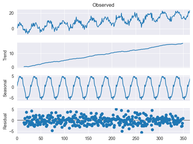
为了进一步理解这一点,请看下面的图片。
我们为什么要做季节性分解?
在我们迈进数学细节,并实现 MQL5 版本季节性分解之前,我们先来了解为什么要在时间序列数据中执行季节性合成。
- 为了检测数据中潜在的形态和趋势
季节性分解能帮助我们识别在原产数据中或许不易察觉的趋势和形态数据,将数据分解为其成分(趋势、季节性、和残差),我们就能更好地理解这些成分如何影响数据的整体行为。 - 去除季节性影响
季节性分解能够用来去除数据中的季节性影响,当我们渴望仅与季节性形态打交道时,这允许我们专注于正在夯实的趋势,或对立因素,例如:当处置气象数据时,展示强烈季节性形态。 - 为了做出准确的预测
当您把数据拆解为成分后,它有助于根据问题过滤那些不太需要的多余信息,例如尝试预测趋势时,仅用趋势信息替代季节性数据更明智。 - 为了比较不同时期或区域的趋势
季节性分解能用来比较不同时间段或区域的趋势,提供不同因素如何影响数据的洞察力。例如,如果我们比较不同区域的零售销售数据,季节性分解能帮助我们识别季节性形态的区域差异,并相应地调整我们的分析。
实现季节性分解的 MQL5 版的
为了实现该分析算法,我们先生成一些简单的随机数据,包含趋势特征、季节性形态、和一些噪声,这在现实数据场景中也能见到,尤其是在外汇和股市当中,其数据并不直接明了和干净。
我们将用 Python 编程语言完成这项任务。
文件: seasonal_decomposition_visualization.ipynb
import pandas as pd
import numpy as np
import seaborn as sns
import matplotlib.pyplot as plt
import os

sns.set_style("darkgrid")

# Create synthetic time-series data
np.random.seed(42)
time = np.arange(0, 365)  # 1 year (daily data)
trend = 0.05 * time  # Linear upward trend
seasonality = 5 * np.sin(2 * np.pi * time / 30)  # 30-day periodic seasonality
noise = np.random.normal(scale=2, size=len(time))  # Random noise

# Combine components to form the time-series
time_series = trend + seasonality + noise

# Plot the original time-series
plt.figure(figsize=(10, 4))
plt.plot(time, time_series, label="Original Time-Series", color="blue")
plt.xlabel("Time (Days)")
plt.ylabel("Value")
plt.title("Synthetic Time-Series with Trend and Seasonality")
plt.legend()
plt.show()
成果
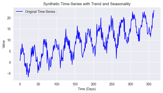
我们知道股市比这复杂得多,但给出的这些简单数据,是让我们尝试从添加的时间序列中揭示 30 天季节性形态、整体趋势,并过滤数据中的一些杂音。
趋势提取
为了提取趋势特征,我们能利用移动平均线(MA),在于它从固定窗口内取平均值来平滑时间序列。这有助于过滤短期波动,高亮潜在趋势。
在加法分解中,趋势是采用季节性周期 p为窗口的移动平均值来估算。

其中:
![]() = 在时间 t 处的趋势成分。
= 在时间 t 处的趋势成分。
![]() = 窗口大小、或季节性周期。
= 窗口大小、或季节性周期。
![]() = 季节性周期的一半。
= 季节性周期的一半。
![]() = 观测到的时间序列值。
= 观测到的时间序列值。
对于乘法分解,我们取几何中值。

其中:
这或许看着像复杂的数学,但几行 MQL5 代码就能拆解它。
vector moving_average(const vector &v, uint k, ENUM_VECTOR_CONVOLVE mode=VECTOR_CONVOLVE_VALID)
 {
   vector kernel = vector::Ones(k) /  k;
   vector ma = v.Convolve(kernel, mode);

   return ma;
 }
我们基于卷积法计算移动平均,因为它灵活高效,并且能处理数组边缘的缺失值,这不同于采用滚动窗口方式计算移动平均。
我们最终公式如下。
//--- compute the trend

   int n = (int)timeseries.Size();
   res.trend = moving_average(timeseries, period);

   // We align trend array with the original series length

   int pad = (int)MathFloor((n - res.trend.Size()) / 2.0);
   int pad_array[] = {pad, n-(int)res.trend.Size()-pad};

   res.trend = Pad(res.trend, pad_array, edge);
季节性成分提取
季节性成分提取是指按给定间隔,隔离时间序列中出现的重复形态,例如:每天、每月、每年、等等。
计算该成分要从原始时间序列数据中去除趋势,根据模型是加法还是乘法,提取方式有所不同。
加法模型
在估测趋势后![]() ,去趋势化序列的计算如下。
,去趋势化序列的计算如下。
其中:
![]() = 在时间 t 处的去趋势数值。
= 在时间 t 处的去趋势数值。
![]() = 在时间 t 处的时间序列值。
= 在时间 t 处的时间序列值。
![]() = 时间 t 处的趋势成分。
= 时间 t 处的趋势成分。
为了计算季节性成分,我们取涵盖季节区间 p 的完整周期计算去趋势的平均值。

其中:
![]() = 数据集中完整季节性周期的数量。
= 数据集中完整季节性周期的数量。
![]() = 季节性周期(例如,月度周期中有 30 个每日数据)。
= 季节性周期(例如,月度周期中有 30 个每日数据)。
![]() = 提取的季节性成分。
= 提取的季节性成分。
乘法模型
当遇到乘法模型,我们用除法替代减法,计算去趋势时间序列。

提取季节性成分是取几何均值,替代算术均值。

这有助于预防由模型乘法特性带来的乖离。
我们如下实现该函数的 MQL5 版本。
//--- compute the seasonal component

   if (model == multiplicative)
     {
       for (ulong i=0; i<timeseries.Size(); i++)
         if (timeseries[i]<=0)
            {
               printf("Error, Multiplicative seasonality is not appropriate for zero and negative values");
               return res;
            }
     }

   vector detrended = {};
   vector seasonal = {};

   switch(model)
     {
      case  additive:
        {
          detrended = timeseries - res.trend;
          seasonal = vector::Zeros(period);

          for (uint i = 0; i < period; i++)
            seasonal[i] = SliceStep(detrended, i, period).Mean(); //Arithmetic mean over cycles
        }
        break;
      case  multiplicative:
        {
          detrended = timeseries / res.trend;
          seasonal = vector::Zeros(period);

          for (uint i = 0; i < period; i++)
            seasonal[i] = MathExp(MathLog(SliceStep(detrended, i, period)).Mean()); //Geometric mean
        }
        break;
      default:
        printf("Unknown model for seasonal component calculations");
        break;
     }


    vector seasonal_repeated = Tile(seasonal, (int)MathFloor(n/period)+1);
    res.seasonal = Slice(seasonal_repeated, 0, n);
Pad 函数会在向量周围添加填充值(额外值),类似于 Numpy.pad,在该场景下它有助于确保移动平均值居中。
   if (model == multiplicative)
     {
       for (ulong i=0; i<timeseries.Size(); i++)
         if (timeseries[i]<=0)
            {
               printf("Error, Multiplicative seasonality is not appropriate for zero and negative values");
               return res;
            }
     }
Tile 函数多次重复季节性向量来构造一个大向量。该过程对于捕捉时间序列中重复的季节性形态至关重要。
残差计算
最后,我们通过减去趋势和季节性来计算残差。
对于加法模型:
![]()
对于乘法模型:

其中:
![]() = 时间 t 处的原始时间序列值。
= 时间 t 处的原始时间序列值。
![]() = 时间 t 处的趋势值。
= 时间 t 处的趋势值。
![]() = 时间 t 的季节性数值。
= 时间 t 的季节性数值。
把所有都放如一个函数
类似于 seasonal_decompose 函数,我从中汲取到灵感,我必须把所有计算挟裹在一个名为 seasonal_decompose 的函数中,其返回一个包含趋势、季节性、和残差向量的结构。
enum seasonal_model { additive, multiplicative }; struct seasonal_decompose_results { vector trend; vector seasonal; vector residuals; }; seasonal_decompose_results seasonal_decompose(const vector ×eries, uint period, seasonal_model model=additive) { seasonal_decompose_results res; if (timeseries.Size() < period) { printf("%s Error: Time series length is smaller than the period. Cannot compute seasonal decomposition.",__FUNCTION__); return res; } //--- compute the trend int n = (int)timeseries.Size(); res.trend = moving_average(timeseries, period); // We align trend array with the original series length int pad = (int)MathFloor((n - res.trend.Size()) / 2.0); int pad_array[] = {pad, n-(int)res.trend.Size()-pad}; res.trend = Pad(res.trend, pad_array, edge); //--- compute the seasonal component if (model == multiplicative) { for (ulong i=0; i<timeseries.Size(); i++) if (timeseries[i]<=0) { printf("Error, Multiplicative seasonality is not appropriate for zero and negative values"); return res; } } vector detrended = {}; vector seasonal = {}; switch(model) { case additive: { detrended = timeseries - res.trend; seasonal = vector::Zeros(period); for (uint i = 0; i < period; i++) seasonal[i] = SliceStep(detrended, i, period).Mean(); //Arithmetic mean over cycles } break; case multiplicative: { detrended = timeseries / res.trend; seasonal = vector::Zeros(period); for (uint i = 0; i < period; i++) seasonal[i] = MathExp(MathLog(SliceStep(detrended, i, period)).Mean()); //Geometric mean } break; default: printf("Unknown model for seasonal component calculations"); break; } vector seasonal_repeated = Tile(seasonal, (int)MathFloor(n/period)+1); res.seasonal = Slice(seasonal_repeated, 0, n); //--- Compute Residuals if (model == additive) res.residuals = timeseries - res.trend - res.seasonal; else // Multiplicative res.residuals = timeseries / (res.trend * res.seasonal); return res; }
我们终能测试该函数了。
为了用乘法模型测试季节性分解,我还要生成正数值,并把它们保存到 CSV 文件之中。
文件: seasonal_decomposition_visualization.ipynb
# Create synthetic time-series data
np.random.seed(42)
time = np.arange(0, 365)  # 1 year (daily data)
trend = 0.05 * time  # Linear upward trend
seasonality = 5 * np.sin(2 * np.pi * time / 30)  # 30-day periodic seasonality
noise = np.random.normal(scale=2, size=len(time))  # Random noise

# Combine components to form the time-series
time_series = trend + seasonality + noise

# Fix for multiplicative decomposition: Shift the series to make all values positive
min_value = np.min(time_series)
if min_value <= 0:
    shift_value = abs(min_value) + 1  # Ensure strictly positive values
    time_series_shifted = time_series + shift_value
else:
    time_series_shifted = time_series
ts_pos_df = pd.DataFrame({
    "timeseries": time_series_shifted
})

ts_pos_df.to_csv(os.path.join(files_path,"pos_ts_df.csv"), index=False)
在我们的 MQL5 脚本内,我们用到在这篇文章中讨论过的数据帧函数库来加载两个时间序列数据集,并在数据加载后运行季节性分解算法。
文件: seasonal_decompose test.mq5
#include <MALE5\Stats Models\Tsa\Seasonal Decompose.mqh>
#include <MALE5\pandas.mqh>
//+------------------------------------------------------------------+
//| Script program start function                                    |
//+------------------------------------------------------------------+
void OnStart()
  {
//--- Additive model

   CDataFrame df;
   df.FromCSV("ts_df.csv");

   vector time_series = df["timeseries"];

//---

    seasonal_decompose_results res_ad = seasonal_decompose(time_series, 30, additive);

    df.Insert("original", time_series);
    df.Insert("trend",res_ad.trend);
    df.Insert("seasonal",res_ad.seasonal);
    df.Insert("residuals",res_ad.residuals);

    df.ToCSV("seasonal_decomposed_additive.csv");

//--- Multiplicative model

   CDataFrame pos_df;
   pos_df.FromCSV("pos_ts_df.csv");

   time_series = pos_df["timeseries"];

//---

    seasonal_decompose_results res_mp = seasonal_decompose(time_series, 30, multiplicative);

    pos_df.Insert("original", time_series);
    pos_df.Insert("trend",res_mp.trend);
    pos_df.Insert("seasonal",res_mp.seasonal);
    pos_df.Insert("residuals",res_mp.residuals);

    pos_df.ToCSV("seasonal_decomposed_multiplicative.csv");
  }
为了用 Python 做可视化,我不得不把成果保存到新的 CSV 文件。
使用加法模型成果绘制的季节性分解
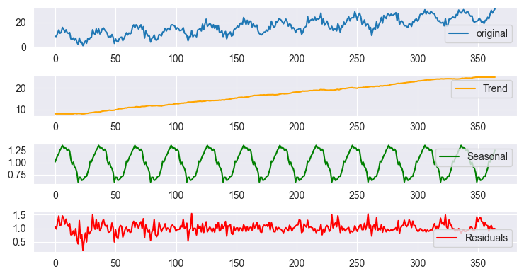
使用乘法模型成果绘制的季节性分解

由于尺度不同,这些绘图看起来几乎相似,但当您查看数据时,成果却有所差别。这和您使用 Python 的统计模型提供的 tsa.seasonal.seasonal_decompose 得到的成果一样。
既然我们已有了季节性分解函数,我们来用它来分析股市。
观察股市中的形态
在分析股市时,识别趋势往往直截了当,尤其是对于那些历史悠久、且基本面强劲的公司。许多大型、财务稳定的公司,由于持续增长、创新和市场需求,倾向于随着时间保持上升轨迹。
然而,在股票价格中检测出季节性形态则更具挑战性。不同于趋势,季节性指的是在固定间隔内反复出现的价格走势,或许其并非总是显而易见,这些形态可能发生在不同的时间帧。
日内季节性
在交易日内的某些钟点或许会出现重复的价格行为(例如,开盘或收盘时波动性增加)。
月度或季度季节性
基于财报报告、经济状况、或投资者情绪,股票价格或许会伴随周期变化。
长期季节性
由于经济周期、或公司特定因素,一些股票多年来展现出重复趋势。
案例研究,苹果公司(AAPL)股票
以苹果公司股票为例,我们可以假设季节性形态每 22 个交易日出现一次,这大约相当于年度数据集中的一个交易月度。该假设基于每月大约有 22 个交易日(不包括周末和节假日)的事实。
应用季节性分解技术,我们就能分析苹果公司股票是否每 22 天展现一次重复性价格走势。如果存在强烈的季节性成分,则表明价格波动或许遵循可预测的周期,这对交易者和分析师很实用;然而,如果未检测到显著的季节性,则价格走势或许主要由外部因素、噪音、或盛行趋势驱动。
我们收集 1000 根柱线的日线收盘价,并按 22 天周期执行乘法季节性分解。
#include <MALE5\Stats Models\Tsa\Seasonal Decompose.mqh>
#include <MALE5\pandas.mqh>

input uint bars_total = 1000;
input uint period_ = 22;
//+------------------------------------------------------------------+
//| Script program start function                                    |
//+------------------------------------------------------------------+
void OnStart()
  {
//---

    vector close, time;
    close.CopyRates(Symbol(), PERIOD_D1, COPY_RATES_CLOSE, 1, bars_total); //closing prices
    time.CopyRates(Symbol(), PERIOD_D1, COPY_RATES_TIME, 1, bars_total); //time

    seasonal_decompose_results res_ad = seasonal_decompose(close, period_, multiplicative);

    CDataFrame df; //A dataframe object for storing the seasonal decomposition outcome

    df.Insert("time", time);
    df.Insert("close", close);
    df.Insert("trend",res_ad.trend);
    df.Insert("seasonal",res_ad.seasonal);
    df.Insert("residuals",res_ad.residuals);

    df.ToCSV(StringFormat("%s.%s.period=%d.seasonal_dec.csv",Symbol(), EnumToString(PERIOD_D1), period_));
  }
出产随后在 Jupyter 笔记簿中调用 stock_market dec.ipynb 进行可视化,如下所示。
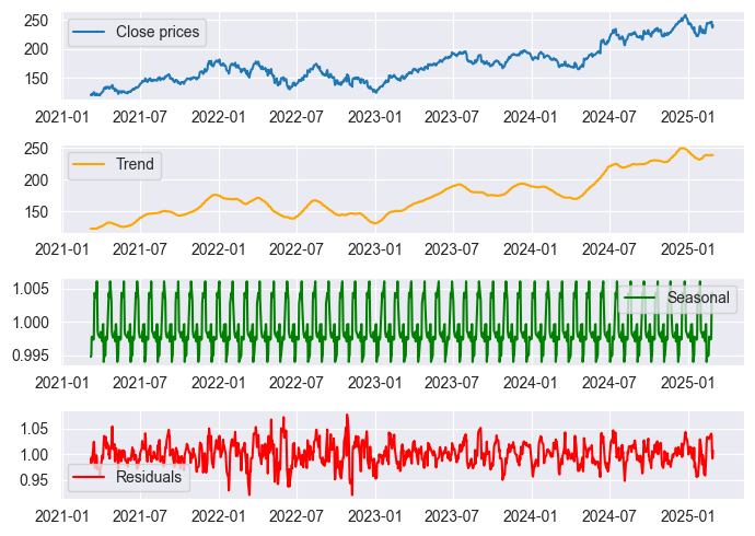
好了,我们能在上面的图表中见到一些季节性形态,但我们无法百分之百确定季节性形态,因为总会有一些误差,挑战在于如何解读这些误差值,并据此进行分析。
基于残差图,我们能见到 2020 年至 2022 年间残差值出现峰值,我们都知道那是全球疫情流行期,故季节性形态或许被打乱、且不一致,示意我们不能信任那段时间的季节性形态。
经验法则。
优良分解:残差应当看起来像随机噪声(白噪声)。
不良分解:残差仍展现出可见结构(未被去除的趋势或季节性效应)。
我们能用不同的数学计数来可视化残差,譬如:
分布图

我们有一个正态分布的残差图,这是一个好迹象,表明苹果公司股票可能存在一些月度形态。
中值与标准差
在加法模型中,残差中值应接近 0,这意味着大多变异可按趋势和季节性解释。
在乘法模型中,残差中值理想情况下接近 1,意味着原始序列可很好地按趋势和季节性解释。
标准差值必须很小
print("Residual Mean:", residuals.mean())  # Should be close to 0
print("Residual Std Dev:", residuals.std())  # Should be small
输出
Residual Mean: 1.0002367590572043
Residual Std Dev: 0.021749969975933727
最后,我们把所有放进一个指标内。
#property indicator_separate_window
#property indicator_buffers 2
#property indicator_plots 1

#property indicator_color1 clrDodgerBlue
#property indicator_style1 STYLE_SOLID
#property indicator_type1 DRAW_LINE
#property indicator_width1 2

//+------------------------------------------------------------------+

double trend_buff[];
double seasonal_buff[];

#include <MALE5\Stats Models\Tsa\Seasonal Decompose.mqh>
#include <MALE5\pandas.mqh>

input uint bars_total = 10000;
input uint period_ = 22;
input ENUM_COPY_RATES price = COPY_RATES_CLOSE;

//+------------------------------------------------------------------+
//| Custom indicator initialization function                         |
//+------------------------------------------------------------------+
int OnInit()
  {
//--- indicator buffers mapping

   SetIndexBuffer(0, seasonal_buff, INDICATOR_DATA);
   SetIndexBuffer(1, trend_buff, INDICATOR_CALCULATIONS);

//---

   IndicatorSetString(INDICATOR_SHORTNAME, "Seasonal decomposition("+string(period_)+")");
   PlotIndexSetString(1, PLOT_LABEL, "seasonal ("+string(period_)+")");

   PlotIndexSetDouble(0, PLOT_EMPTY_VALUE, 0.0);

   ArrayInitialize(seasonal_buff, EMPTY_VALUE);
   ArrayInitialize(trend_buff, EMPTY_VALUE);

   return(INIT_SUCCEEDED);
  }

//+------------------------------------------------------------------+
//| Custom indicator iteration function                              |
//+------------------------------------------------------------------+
int OnCalculate(const int rates_total,
                const int prev_calculated,
                const datetime &time[],
                const double &open[],
                const double &high[],
                const double &low[],
                const double &close[],
                const long &tick_volume[],
                const long &volume[],
                const int &spread[])
  {
//---

    if (prev_calculated==rates_total) //not on a new bar, calculate the indicator on the opening of a new bar
      return rates_total;

    ArrayInitialize(seasonal_buff, EMPTY_VALUE);
    ArrayInitialize(trend_buff, EMPTY_VALUE);

//---

    Comment("rates total: ",rates_total," bars total: ",bars_total);

    //if (rates_total<(int)bars_total)
    //  return rates_total;

    vector close_v;
    close_v.CopyRates(Symbol(), Period(), price, 0, bars_total); //closing prices

    seasonal_decompose_results res = seasonal_decompose(close_v, period_, multiplicative);

    for (int i=MathAbs(rates_total-(int)bars_total), count=0; i<rates_total; i++, count++) //calculate only the chosen number of bars
      {
         trend_buff[i] = res.trend[count];
         seasonal_buff[i] = res.seasonal[count];
      }

//--- return value of prev_calculated for next call
   return(rates_total);
  }
由于季节性分解计算的性质,当我们使用图表中所有可用的汇率时,计算可能较为昂贵。一旦图表上出现新的汇率,我们不得不约束用于计算和绘制的柱线数量。
我只得创建两个分离的指标,其一用于绘制季节性形态,另一个按同样逻辑绘制残差。
以下是据苹果公司的指示绘图。
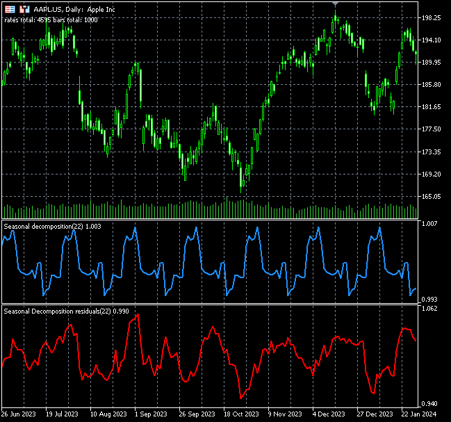
该指标的季节性形态也可解读为交易信号、或超卖超买条件,如上图所见,目前难以言表,因为我尚未立足交易一侧探讨它。我鼓励您把它当家庭作业来做。
后记
在您的算法交易工具箱中,季节性分解是一种实用的技术,一些数据科研者基于手头的时间序列数据,用它来创造新特征,另一些则用它来分析数据的性质,然后针对特定问题决定采用合适的机器学习技术,这就引出了一个重要问题:何时使用季节性分解?
一些数据科研者先从执行季节性分解开始,将时间序列拆解为其底层成分:趋势、季节性、和残差。如果数据中存在明显的季节性形态,则会采用季节性指数平滑(也称为季节性 Holt-Winters 方法)来尝试预测数据;但如果没有明确的季节性形态,或者季节性形态较弱、或不规则,则会部署 ARIMA 模型和其它标准机器学习模型,尝试揭示时间序列数据中的形态,并做出预测。
附表
| 文件名 & 路径 | 说明 & 用法 |
|---|---|
| Include\pandas.mqh | 由 Dataframe 类组成,用于存储和操纵 Pandas 格式的数据。 |
| Include\Seasonal Decompose.mqh | 包含所有季节性分解函数的 MQL5 代码行。 |
| Indicators\Seasonal Decomposition.mq5 | 该指标绘制季节性成分图。 |
| Indicators\Seasonal Decomposition residuals.mq5 | 该指标绘制残差成分图。 |
| Scripts\seasonal_decompose test.mq5 | 一个简单的脚本,用于实现和调试季节性分解函数、及其成分。 |
| Scripts\stock market seasonal dec.mq5 | 分析品种收盘价,并将结果保存到 CSV 文件,以供后续分析的脚本 |
| Python\seasonal_decomposition_visualization.ipynb | 从 CSV 文件中可视化季节性分解结果的 Jupyter 笔记簿。 |
| Python\stock_market seasonal dec.ipynb | 可视化股票季节性分解结果的 Jupyter 笔记簿。 |
| Files\*.csv | 包含季节性分解结果的数据 CSV 文件,来自 Python 代码和 MQL5 两者。 |
本文由MetaQuotes Ltd译自英文
原文地址: https://www.mql5.com/en/articles/17361
注意: MetaQuotes Ltd.将保留所有关于这些材料的权利。全部或部分复制或者转载这些材料将被禁止。
本文由网站的一位用户撰写,反映了他们的个人观点。MetaQuotes Ltd 不对所提供信息的准确性负责,也不对因使用所述解决方案、策略或建议而产生的任何后果负责。
