
Data Science and ML (Part 33): Pandas Dataframe in MQL5, Data Collection for ML Usage made easier

Contents
- Introduction
- Basic Data Structures in Pandas
- A Pandas Dataframe
- Adding Data Into the Dataframe Class
- Assigning a CSV file to the Dataframe
- Visualizing What's in the Dataframe
- Exporting the Dataframe To a CSV file
- Dataframe Selection and Indexing
- Exploring and Inspecting Pandas Dataframe
- Time Series and Data Transformation Methods
- Collecting Data for Machine Learning
- Training a Machine Learning Model
- Deploying a Machine Learning Model in MQL5
- Conclusion
Introduction
When it comes to working with machine learning models, it is essential that we have the same data structure if not the same values for all the environments; Training, validation, and testing. With Open Neural Network Exchange (ONNX) models being supported in MQL5 and MetaTrader 5, nowadays we have an opportunity to import models trained outside into the MQL5 language and use them for trading purposes.
Since most users use Python for training these Artificial Intelligence (AI) models which are then being deployed in MetaTrader 5 through MQL5 code, there could be a huge difference in how the data is organized, and often times even the values within the same data structure can be slightly different, this is due to the difference in the two technologies.

In this article, we are going to mimic the Pandas library available in Python language. It is one of the most popular libraries, useful particularly when it comes to working with vast amounts of data.
Since this library is used by data scientists to prepare and manipulate data used in training ML models, by harnessing its ability, we aim to have the same data playground in MQL5 as in Python.
Basic Data Structures in Pandas
The Pandas library provides two types of classes for handling data.
- Series: a one-dimensional labeled array for holding data of any type such as integers, strings, Objects, etc.
s = pd.Series([1, 3, 5, np.nan, 6, 8])
- Dataframe: a two-dimensional data structure that holds data like a two-dimensional array or a table with rows and columns.
Since a series pandas data class is one-dimensional, It is more like an Array or a vector in MQL5, we are not going to work on it. Our focus is on the two-dimensional "Dataframe".
A Pandas DataFrame
Again, this data structure holds data like a two-dimensional array or a table with rows and columns, in MQL5 we can have a two-dimensional array but, the most practical two-dimensional object we can use for this task is a matrix.
Since we now know that at the core of the Pandas Dataframe lies a two-dimensional array, we can implement this similar foundation in our Pandas class in MQL5.
File: pandas.mqh
class CDataFrame
  {
public:

                     string m_columns[]; //An array of string values for keeping track of the column names
                     matrix m_values; // A 2D matrix

                     CDataFrame();
                    ~CDataFrame(void);
 }
We need to have an array named "m_columns" for storing the column names for every column in the Dataframe, unlike other libraries for working with data like Numpy, Pandas ensures the data stored is human-friendly by keeping track of the column names.
Pandas Datafrme in Python supports different data types such as Integers, strings, objects, etc.
import pandas as pd

df = pd.DataFrame({
    "Integers": [1,2,3,4,5],
    "Doubles": [0.1,0.2,0.3,0.4,0.5],
    "Strings": ["one","two","three","four","five"]
})
We are not going to implement this same flexibility in our MQL5 library because the goal of this library is to aid us when working with machine learning models where variables of float and double data type are the most useful.
So, make sure you cast (integers, long, ulong etc) into values of double data type and encode all (string) variables you have before plugging them into the Dataframe class because all variables will be forced to become of double data type.
Adding Data Into the Dataframe Class
Now that we know that a matrix at the core of a Dataframe object is the one responsible for storing all the data, Let us implement ways to add information to it.
In Python, you can simply create a new Dataframe and add objects to it by calling the method;
df = pd.DataFrame({
    "first column": [1,2,3,4,5],
    "second column": [10,20,30,40,50]
})
Due to the MQL5 language syntax, we can't have a class or method behave like this, Let's implement a method known as Insert.
File: pandas.mqh
void CDataFrame::Insert(string name, const vector &values)
 {
//--- Check if the column exists in the m_columns array if it does exists, instead of creating a new column we modify an existing one

   int col_index = -1;

   for (int i=0; i<(int)m_columns.Size(); i++)
     if (name == m_columns[i])
       {
         col_index = i;
         break;
       }

//---  We check if the dimensiona are Ok

   if (m_values.Rows()==0)
     m_values.Resize(values.Size(), m_values.Cols());

   if (values.Size() > m_values.Rows() && m_values.Rows()>0) //Check if the new column has a bigger size than the number of rows present in the matrix
    {
      printf("%s new column '%s' size is bigger than the dataframe",__FUNCTION__,name);
      return;
    }

//---

   if (col_index != -1)
    {
       m_values.Col(values, col_index);
       if (MQLInfoInteger(MQL_DEBUG))  printf("%s column '%s' exists, It will be modified",__FUNCTION__,name);
       return;
    }

//--- If a given vector to be added to the dataframe is smaller than the number of rows present in the matrix, we fill the remaining values with Not a Number (NaN)

   vector temp_vals = vector::Zeros(m_values.Rows());
   temp_vals.Fill(NaN); //to create NaN values when there was a dimensional mismatch

     for (ulong i=0; i<values.Size(); i++)
       temp_vals[i] = values[i];

//---

   m_values.Resize(m_values.Rows(), m_values.Cols()+1); //We resize the m_values matrix to accomodate the new column
   m_values.Col(temp_vals, m_values.Cols()-1);     //We insert the new column after the last column

   ArrayResize(m_columns, m_columns.Size()+1); //We increase the sice of the column names to accomodate the new column name
   m_columns[m_columns.Size()-1] = name;   //we assign the new column to the last place in the array
 }
We can parse new information to the Dataframe as follows;
#include <MALE5\pandas.mqh>
//+------------------------------------------------------------------+
//| Script program start function                                    |
//+------------------------------------------------------------------+
void OnStart()
  {
//---

    CDataFrame df;

    vector v1= {1,2,3,4,5};
    vector v2= {10,20,30,40,50};

    df.Insert("first column", v1);
    df.Insert("second column", v2);
  }
Alternatively, we can give the class constructur the ability to receive a matrix and its column names.
CDataFrame::CDataFrame(const string &columns, const matrix &values)
 {
   string columns_names[]; //A temporary array for obtaining column names from a string
   ushort sep = StringGetCharacter(",", 0);
   if (StringSplit(columns, sep, columns_names)<0)
     {
       printf("%s failed to obtain column names",__FUNCTION__);
       return;
     }

   if (columns_names.Size() != values.Cols()) //Check if the given number of column names is equal to the number of columns present in a given matrix
     {
       printf("%s dataframe's columns != columns present in the values matrix",__FUNCTION__);
       return;
     }

   ArrayCopy(m_columns, columns_names); //We assign the columns to the m_columns array
   m_values = values; //We assing the given matrix to the m_values matrix
 }
We can also add new information to the Dataframe class as follows;
void OnStart()
  {
//---

    matrix data = {
      {1,10},
      {2,20},
      {3,30},
      {4,40},
      {5,50},
    };


    CDataFrame df("first column,second column",data);
  }
I suggest you use the Insert method for adding data to the Dataframe class that any other method for the task.
The prior two discussed methods are useful when you are preparing datasets, we also need a function for loading the data present in a dataset.
Assigning a CSV file to the Dataframe
The method for reading a CSV file and assigning the values to a Dataframe is among the most useful functions in Pandas when you are working with the library in Python.
df = pd.read_csv("EURUSD.PERIOD_D1.csv")
Let us implement this method in our MQL5 class;
bool CDataFrame::ReadCSV(string file_name,string delimiter=",",bool is_common=false, bool verbosity=false)
  {
   matrix mat_ = {};
   int rows_total=0;
   int handle = FileOpen(file_name,FILE_READ|FILE_CSV|FILE_ANSI|(is_common?FILE_IS_COMMON:FILE_ANSI),delimiter); //Open a csv file

   ResetLastError();
   if(handle == INVALID_HANDLE) //Check if the file handle is ok if not return false
     {
      printf("Invalid %s handle Error %d ",file_name,GetLastError());
      Print(GetLastError()==0?" TIP | File Might be in use Somewhere else or in another Directory":"");

      return false;
     }
   else
     {
      int column = 0, rows=0;

      while(!FileIsEnding(handle))
        {
         string data = FileReadString(handle);
         //---
         if(rows ==0)
           {
            ArrayResize(m_columns,column+1);
            m_columns[column] = data;
           }
         if(rows>0)  //Avoid the first column which contains the column's header
            mat_[rows-1,column] = (double(data)); //add a value to the matrix
         column++;
         //---
         if(FileIsLineEnding(handle)) //At the end of the each line
           {
            rows++;

            mat_.Resize(rows,column); //Resize the matrix to accomodate new values
            column = 0;
           }
        }

      if (verbosity) //if verbosity is set to true, we print the information to let the user know the progress, Useful for debugging purposes
        printf("Reading a CSV file... record [%d]",rows);

      rows_total = rows;
      FileClose(handle); //Close the file after reading it
     }

   mat_.Resize(rows_total-1,mat_.Cols());
   m_values = mat_;

   return true;
  }
Below is how you can read a CSV file and assign it to the Dataframe directly.
void OnStart()
  {
//---

    CDataFrame df;

    df.ReadCSV("EURUSD.PERIOD_D1.csv");

    df.Head();
  }
Visualizing What's in the Dataframe
We have seen how you can add information into a Dataframe but, it is very crucial to be able to briefly look into the Dataframe to see what is it all about. In most cases, you will be working with big Dataframes that often require looking back into the Dataframe for exploration and recalling purposes.
Pandas has a method known as "head" which returns the first n rows for the Dataframe object based on position. This method is useful for quickly testing if your object has the right type of data in it.
When the method "head" is called in a Jupyter Notebook cell with its default value(s), five first rows of the Dataframe are displayed in the cell output.
File: main.ipynb
df = pd.read_csv("EURUSD.PERIOD_D1.csv")

df.head()
Output
| Open | High | Low | Close | |
|---|---|---|---|---|
| 0 | 1.09381 | 1.09548 | 1.09003 | 1.09373 |
| 1 | 1.09678 | 1.09810 | 1.09361 | 1.09399 |
| 2 | 1.09701 | 1.09973 | 1.09606 | 1.09805 |
| 3 | 1.09639 | 1.09869 | 1.09542 | 1.09742 |
| 4 | 1.10302 | 1.10396 | 1.09513 | 1.09757 |
We can make a similar function for the task in MQL5.
void CDataFrame::Head(const uint count=5)
{
   // Calculate maximum width needed for each column
   uint num_cols = m_columns.Size();
   uint col_widths[];
   ArrayResize(col_widths, num_cols);

   for (uint col = 0; col < num_cols; col++) //Determining column width for visualizing a simple table
   {
      uint max_width = StringLen(m_columns[col]);
      for (uint row = 0; row < count && row < m_values.Rows(); row++)
      {
         string num_str = StringFormat("%.8f", m_values[row][col]);
         max_width = MathMax(max_width, StringLen(num_str));
      }
      col_widths[col] = max_width + 4; // Extra padding for readability
   }

   // Print column headers with calculated padding
   string header = "";
   for (uint col = 0; col < num_cols; col++)
   {
      header += StringFormat("| %-*s ", col_widths[col], m_columns[col]);
   }
   header += "|";
   Print(header);

   // Print rows with padding for each column
   for (uint row = 0; row < count && row < m_values.Rows(); row++)
   {
      string row_str = "";
      for (uint col = 0; col < num_cols; col++)
      {
         row_str += StringFormat("| %-*.*f ", col_widths[col], 8, m_values[row][col]);
      }
      row_str += "|";
      Print(row_str);
   }

   // Print dimensions
   printf("(%dx%d)", m_values.Rows(), m_values.Cols());
}
By default, this function displays five first rows in our Dataframe.
void OnStart()
  {
//---

    CDataFrame df;

    df.ReadCSV("EURUSD.PERIOD_D1.csv");

    df.Head();
  }
Outputs
GI      0       12:37:02.983    pandas test (Volatility 75 Index,H1)    | Open           | High           | Low            | Close          |
RH      0       12:37:02.983    pandas test (Volatility 75 Index,H1)    | 1.09381000     | 1.09548000     | 1.09003000     | 1.09373000     |
GI      0       12:37:02.984    pandas test (Volatility 75 Index,H1)    | 1.09678000     | 1.09810000     | 1.09361000     | 1.09399000     |
DI      0       12:37:02.984    pandas test (Volatility 75 Index,H1)    | 1.09701000     | 1.09973000     | 1.09606000     | 1.09805000     |
EI      0       12:37:02.984    pandas test (Volatility 75 Index,H1)    | 1.09639000     | 1.09869000     | 1.09542000     | 1.09742000     |
CI      0       12:37:02.984    pandas test (Volatility 75 Index,H1)    | 1.10302000     | 1.10396000     | 1.09513000     | 1.09757000     |
FE      0       12:37:02.984    pandas test (Volatility 75 Index,H1)    (1000x4)
Exporting the Dataframe To a CSV file
After collecting all different kinds of data into the Dataframe, we need to export it outside MetaTrader 5 where all the machine learning procedures occur.
A CSV file is handy when it comes to exporting data, especially since we will then use the Pandas library to import the CSV file in Python language.
Let us save the Dataframe we extracted from a CSV file back to the CSV file.
In Python.
df.to_csv("EURUSDcopy.csv", index=False) The outcome is a csv file named EURUSDcopy.csv.
Below is an implementation of this method in MQL5.
bool CDataFrame::ToCSV(string csv_name, bool common=false, int digits=5, bool verbosity=false)
  {
   FileDelete(csv_name);
   int handle = FileOpen(csv_name,FILE_WRITE|FILE_SHARE_WRITE|FILE_CSV|FILE_ANSI|(common?FILE_COMMON:FILE_ANSI),",",CP_UTF8); //open a csv file

   if(handle == INVALID_HANDLE) //Check if the handle is OK
     {
       printf("Invalid %s handle Error %d ",csv_name,GetLastError());
       return (false);
     }

//---

   string concstring;
   vector row = {};
   vector colsinrows = m_values.Row(0);

   if (ArraySize(m_columns) != (int)colsinrows.Size())
      {
         printf("headers=%d and columns=%d from the matrix vary is size ",ArraySize(m_columns),colsinrows.Size());
         DebugBreak();
         return false;
      }

//---

   string header_str = "";
   for (int i=0; i<ArraySize(m_columns); i++) //We concatenate the header only separating it with a comma delimeter
      header_str += m_columns[i] + (i+1 == colsinrows.Size() ? "" : ",");

   FileWrite(handle,header_str);
   FileSeek(handle,0, SEEK_SET);

   for(ulong i=0; i<m_values.Rows() && !IsStopped(); i++)
     {
      ZeroMemory(concstring);

      row = m_values.Row(i);
      for(ulong j=0, cols =1; j<row.Size() && !IsStopped(); j++, cols++)
        {
         concstring += (string)NormalizeDouble(row[j],digits) + (cols == m_values.Cols() ? "" : ",");
        }

      if (verbosity) //if verbosity is set to true, we print the information to let the user know the progress, Useful for debugging purposes
        printf("Writing a CSV file... record [%d/%d]",i+1,m_values.Rows());

      FileSeek(handle,0,SEEK_END);
      FileWrite(handle,concstring);
     }

   FileClose(handle);

   return (true);
  }
Below is how to use this method.
void OnStart()
  {
    CDataFrame df;

    df.ReadCSV("EURUSD.PERIOD_D1.csv"); //Assign a csv file into the dataframe

    df.ToCSV("EURUSDcopy.csv"); //Save the dataframe back into a CSV file as a copy
  }
The outcome is the creation of the CSV file with the name EURUSDcopy.csv.
Now that we have discussed about creating a Dataframe, inserting the values into it, importing, and exporting the data, let's see data selection and indexing techniques.
Dataframe Selection and Indexing
It is very crucial to have the ability to slice, select, or access some specific parts of the Dataframe at times. For instance; while using a model to make predictions you might want to access only the latest values (the last row) in the dataframe meanwhile, during training, you may want to access some rows located at the beginning of the Dataframe.
Accessing a Column
To access a column, we can implement an index operator that takes a string values in our class.
vector operator[] (const string index) {return GetColumn(index); } //Access a column by its name
The function "GetColumn" when given a column name, it returns a vector of its values when it is found.
Usage
Print("Close column: ",df["Close"]);
Outputs
2025.01.27 16:16:19.726 pandas test (EURUSD,H1) Close column: [1.09373,1.09399,1.09805,1.09742,1.09757,1.10297,1.10453,1.10678,1.1135,1.11594,1.11765,1.11327,1.11797,1.11107,1.1163,1.11616,1.11177,1.11141,1.11326,1.10745,1.10747,1.10111,1.10192,1.10351,1.10861,1.11106,1.1083,1.10435,1.10723,1.10483,1.1078,1.11199,1.11843,1.1161,1.11932,1.11113,1.11499,1.113,1.10852,1.10267,1.09712,1.10124,1.09928,1.09321,1.09156,1.09188,1.09236,1.09315,1.09511,1.09107,1.07913,1.08258,1.08142,1.08211,1.08551,1.0845,1.08392,1.08529,1.08905,1.08818,1.08959,1.09396,1.08986,
The "loc" Indexing
This indexing helps to access a group or rows and columns by labels(s) or a boolean array.
In Pandas Python.
df.loc[0] Outputs.
Open     1.09381
High     1.09548
Low      1.09003
Close    1.09373
Name: 0, dtype: float64
In MQL5, we can implement this as a regular function.
vector CDataFrame::Loc(int index, uint axis=0)
  {
   if(axis == 0)
     {
      vector row = {};

      //--- Convert negative index to positive

      if(index < 0)
         index = (int)m_values.Rows() + index;

      if(index < 0 || index >= (int)m_values.Rows())
        {
         printf("%s Error: Row index out of bounds. Given index: %d", __FUNCTION__, index);
         return row;
        }

      return m_values.Row(index);
     }
   else
      if(axis == 1)
        {
         vector column = {};

         //--- Convert negative index to positive

         if(index < 0)
            index = (int)m_values.Cols() + index;

         //--- Check bounds

         if(index < 0 || index >= (int)m_values.Cols())
           {
            printf("%s Error: Column index out of bounds. Given index: %d", __FUNCTION__, index);
            return column;
           }

         return m_values.Col(index);
        }
      else
         printf("%s Failed, Unknown axis ",__FUNCTION__);

   return vector::Zeros(0);
  }
I added the argument named axis to gain the ability to choose between obtaining a row (along axis 0) and a column (along axis 1).
When this function receives a negative value it accesses items in reverse, an index value of -1 is the last element in the Dataframe (last row when axis=0, last column when axis=1).
Usage
void OnStart()
  {
//---
    CDataFrame df;

    df.ReadCSV("EURUSD.PERIOD_D1.csv");

    df.Head();
    Print("First row",df.Loc(0));

//---

    Print("Last 5 items in df\n",df.Tail());

    Print("Last row: ",df.Loc(-1));
    Print("Last Column: ",df.Loc(-1, 1));
  }
Outputs
RM      0       09:04:21.355    pandas test (EURUSD,H1) | Open           | High           | Low            | Close          |
IN      0       09:04:21.355    pandas test (EURUSD,H1) | 1.09381000     | 1.09548000     | 1.09003000     | 1.09373000     |
GP      0       09:04:21.355    pandas test (EURUSD,H1) | 1.09678000     | 1.09810000     | 1.09361000     | 1.09399000     |
NS      0       09:04:21.355    pandas test (EURUSD,H1) | 1.09701000     | 1.09973000     | 1.09606000     | 1.09805000     |
IE      0       09:04:21.355    pandas test (EURUSD,H1) | 1.09639000     | 1.09869000     | 1.09542000     | 1.09742000     |
IG      0       09:04:21.355    pandas test (EURUSD,H1) | 1.10302000     | 1.10396000     | 1.09513000     | 1.09757000     |
NJ      0       09:04:21.355    pandas test (EURUSD,H1) (1000x4)
EO      0       09:04:21.355    pandas test (EURUSD,H1) First row[1.09381,1.09548,1.09003,1.09373]
JF      0       09:04:21.355    pandas test (EURUSD,H1) Last 5 items in df
DN      0       09:04:21.355    pandas test (EURUSD,H1) [[1.20796,1.21591,1.20742,1.21416]
JK      0       09:04:21.355    pandas test (EURUSD,H1)  [1.21023,1.21474,1.20588,1.20814]
PR      0       09:04:21.355    pandas test (EURUSD,H1)  [1.21089,1.21342,1.20953,1.21046]
OO      0       09:04:21.355    pandas test (EURUSD,H1)  [1.21281,1.21664,1.20785,1.2109]
FK      0       09:04:21.355    pandas test (EURUSD,H1)  [1.21444,1.21774,1.21101,1.21203]]
EM      0       09:04:21.355    pandas test (EURUSD,H1) Last row: [1.21444,1.21774,1.21101,1.21203]
QM      0       09:04:21.355    pandas test (EURUSD,H1) Last Column: [1.09373,1.09399,1.09805,1.09742,1.09757,1.10297,1.10453,1.10678,1.1135,1.11594,1.11765,1.11327,1.11797,1.11107,1.1163,1.11616,1.11177,1.11141,1.11326,1.10745,1.10747,1.10111,1.10192,1.10351,1.10861,1.11106,1.1083,1.10435,1.10723,1.10483,1.1078,1.11199,1.11843,1.1161,1.11932,1.11113,1.11499,1.113,1.10852,1.10267,1.09712,1.10124,1.09928,1.00063,…]
The "iloc" method
The Iloc function in introduced in our class selects rows and columns of a Dataframe by integer positions similar to the iloc method offered by Pandas in Python.
This method returns a new Dataframe which is a result of the sliced operation.
MQL implementation.
CDataFrame Iloc(ulong start_row, ulong end_row, ulong start_col, ulong end_col);
Usage
df = df.Iloc(0,100,0,3); //Slice from the first row to the 99th from the first column to the 2nd

df.Head();
Outputs
DJ      0       16:40:19.699    pandas test (EURUSD,H1) | Open           | High           | Low            |
LQ      0       16:40:19.699    pandas test (EURUSD,H1) | 1.09381000     | 1.09548000     | 1.09003000     |
PM      0       16:40:19.699    pandas test (EURUSD,H1) | 1.09678000     | 1.09810000     | 1.09361000     |
EI      0       16:40:19.699    pandas test (EURUSD,H1) | 1.09701000     | 1.09973000     | 1.09606000     |
DE      0       16:40:19.699    pandas test (EURUSD,H1) | 1.09639000     | 1.09869000     | 1.09542000     |
FQ      0       16:40:19.699    pandas test (EURUSD,H1) | 1.10302000     | 1.10396000     | 1.09513000     |
GS      0       16:40:19.699    pandas test (EURUSD,H1) (100x3)
The "at" method
This method returns a single value from the Dataframe.
MQL implementation.
double CDataFrame::At(ulong row, string col_name)
  {
   ulong col_number = (ulong)ColNameToIndex(col_name, m_columns);
   return m_values[row][col_number];
  }
Usage.
void OnStart()
  {
//---
    CDataFrame df;

    df.ReadCSV("EURUSD.PERIOD_D1.csv");

    Print(df.At(0,"Close")); //Returns the first value within the Close column
  }
Outputs.
2025.01.27 16:47:16.701 pandas test (EURUSD,H1) 1.09373
The "iat" method
This enables us to access a single value in the Dataframe by position.
MQL implementation.
double CDataFrame::Iat(ulong row,ulong col)
  {
   return m_values[row][col];
  }
Usage
Print(df.Iat(0,0)); //Returns the value at first row and first colum
Output.
2025.01.27 16:53:32.627 pandas test (EURUSD,H1) 1.09381
Dropping columns from the Dataframe using the "drop" method
It sometimes happens that we have unwanted columns in our dataframe, or we want to remove some variables for training purposes. The drop function can help with this task.
MQL implementation.
CDataFrame CDataFrame::Drop(const string cols)
  {
   CDataFrame df;

   string column_names[];
   ushort sep = StringGetCharacter(",",0);
   if(StringSplit(cols, sep, column_names) < 0)
     {
      printf("%s Failed to get the columns, ensure they are separated by a comma. Error = %d", __FUNCTION__, GetLastError());
      return df;
     }

   int columns_index[];
   uint size = column_names.Size();
   ArrayResize(columns_index, size);

   if(size > m_values.Cols())
     {
      printf("%s failed, The number of columns > columns present in the dataframe", __FUNCTION__);
      return df;
     }

// Fill columns_index with column indices to drop
   for(uint i = 0; i < size; i++)
     {
      columns_index[i] = ColNameToIndex(column_names[i], m_columns);
      if(columns_index[i] == -1)
        {
         printf("%s Column '%s' not found in this DataFrame", __FUNCTION__, column_names[i]);
         //ArrayRemove(column_names, i, 1);
         continue;
        }
     }

   matrix new_data(m_values.Rows(), m_values.Cols() - size);
   string new_columns[];
   ArrayResize(new_columns, (int)m_values.Cols() - size);

// Populate new_data with columns not in columns_index
   for(uint i = 0, count = 0; i < m_values.Cols(); i++)
     {
      bool to_drop = false;
      for(uint j = 0; j < size; j++)
        {
         if(i == columns_index[j])
           {
            to_drop = true;
            break;
           }
        }

      if(!to_drop)
        {
         new_data.Col(m_values.Col(i), count);
         new_columns[count] = m_columns[i];
         count++;
        }
     }

// Replace original data with the updated matrix and columns

   df.m_values = new_data;
   ArrayResize(df.m_columns, new_columns.Size());
   ArrayCopy(df.m_columns, new_columns);

   return df;
  }
Usage
void OnStart()
  {
//---
    CDataFrame df;

    df.ReadCSV("EURUSD.PERIOD_D1.csv");

    CDataFrame new_df = df.Drop("Open,Close"); //drop the columns and assign the dataframe to a new object

    new_df.Head();
  }
Outputs
II      0       19:18:22.997    pandas test (EURUSD,H1) | High           | Low            |
GJ      0       19:18:22.997    pandas test (EURUSD,H1) | 1.09548000     | 1.09003000     |
EP      0       19:18:22.998    pandas test (EURUSD,H1) | 1.09810000     | 1.09361000     |
CF      0       19:18:22.998    pandas test (EURUSD,H1) | 1.09973000     | 1.09606000     |
RL      0       19:18:22.998    pandas test (EURUSD,H1) | 1.09869000     | 1.09542000     |
MR      0       19:18:22.998    pandas test (EURUSD,H1) | 1.10396000     | 1.09513000     |
DH      0       19:18:22.998    pandas test (EURUSD,H1) (1000x2)
Now that we have functions for indexing and selecting some parts of the Dataframe, let's implement several Pandas functions to help us with data exploration and inspection.
Exploring and Inspecting Pandas Dataframe
The "tail" function
This method displays the last few rows of the Dataframe.
MQL5 implementation.
matrix CDataFrame::Tail(uint count=5)
  {
   ulong rows = m_values.Rows();
   if(count>=rows)
     {
      printf("%s count[%d] >= number of rows in the df[%d]",__FUNCTION__,count,rows);
      return matrix::Zeros(0,0);
     }

   ulong start = rows-count;
   matrix res = matrix::Zeros(count, m_values.Cols());

   for(ulong i=start, row_count=0; i<rows; i++, row_count++)
      res.Row(m_values.Row(i), row_count);

   return res;
  }
Usage.
void OnStart()
  {
//---
    CDataFrame df;

    df.ReadCSV("EURUSD.PERIOD_D1.csv");

    Print(df.Tail());
  }
By default, the function returns 5 last rows of the Dataframe.
GR      0       17:06:42.044    pandas test (EURUSD,H1) [[1.20796,1.21591,1.20742,1.21416]
MG      0       17:06:42.044    pandas test (EURUSD,H1)  [1.21023,1.21474,1.20588,1.20814]
KQ      0       17:06:42.044    pandas test (EURUSD,H1)  [1.21089,1.21342,1.20953,1.21046]
DK      0       17:06:42.044    pandas test (EURUSD,H1)  [1.21281,1.21664,1.20785,1.2109]
MO      0       17:06:42.044    pandas test (EURUSD,H1)  [1.21444,1.21774,1.21101,1.21203]]
The "info" Function
This function is very useful in understanding the structure of the Dataframe, data types, memory usage, and the presence of not-null values.
Below is its MQL5 implementation.
void CDataFrame::Info(void)
Outputs.
ES      0       17:34:04.968    pandas test (EURUSD,H1) <class 'CDataFrame'>
IH      0       17:34:04.968    pandas test (EURUSD,H1) RangeIndex: 1000 entries, 0 to 999
LR      0       17:34:04.968    pandas test (EURUSD,H1) Data columns (total 4 columns):
PD      0       17:34:04.968    pandas test (EURUSD,H1)  #   Column    Non-Null Count   Dtype
OQ      0       17:34:04.968    pandas test (EURUSD,H1) ---  ------    --------------   -----
FS      0       17:34:04.968    pandas test (EURUSD,H1)  0   Open      1000 non-null    double
GH      0       17:34:04.968    pandas test (EURUSD,H1)  1   High      1000 non-null    double
LS      0       17:34:04.968    pandas test (EURUSD,H1)  2   Low       1000 non-null    double
IH      0       17:34:04.968    pandas test (EURUSD,H1)  3   Close     1000 non-null    double
FJ      0       17:34:04.968    pandas test (EURUSD,H1) memory usage: 31.2 KB
The "describe" Function
This function provides descriptive statistics for all the numeric columns in a Dataframe. The information it provides includes, the Mean, Standard deviation, the count, minimum value, and maximum value of the columns not to menthion the 25%, 50%, and 75% percentile values of each column.
Below is the overview of how the function was implemented in MQL5.
void CDataFrame::Describe(void)
Usage
void OnStart()
  {
//---
    CDataFrame df;

    df.ReadCSV("EURUSD.PERIOD_D1.csv");

    //Print(df.Tail());
    df.Describe();
  }
Outputs.
MM      0       18:10:42.459    pandas test (EURUSD,H1)            Open      High      Low       Close
JD      0       18:10:42.460    pandas test (EURUSD,H1) count      1000      1000      1000      1000
HD      0       18:10:42.460    pandas test (EURUSD,H1) mean       1.104156  1.108184  1.100572  1.104306
HM      0       18:10:42.460    pandas test (EURUSD,H1) std        0.060646  0.059900  0.061097  0.060507
NQ      0       18:10:42.460    pandas test (EURUSD,H1) min        0.959290  0.967090  0.953580  0.959320
DI      0       18:10:42.460    pandas test (EURUSD,H1) 25%        1.069692  1.073520  1.066225  1.069950
DE      0       18:10:42.460    pandas test (EURUSD,H1) 50%        1.090090  1.093640  1.087100  1.090385
FN      0       18:10:42.460    pandas test (EURUSD,H1) 75%        1.142937  1.145505  1.139295  1.142365
CG      0       18:10:42.460    pandas test (EURUSD,H1) max        1.232510  1.234950  1.226560  1.232620
Getting the Dataframe Shape and Columns Present in the Dataframe
Pandas in Python have methods such as pandas.DataFrame.shape which returns the shape of the Dataframe, and pandas.DataFrame.columns which return the columns present in the Dataframe.
In our class, we can access these values from a globally defined matrix named m_values as follows.
printf("df shape = (%dx%d)",df.m_values.Rows(),df.m_values.Cols());
Outputs.
2025.01.27 18:24:14.436 pandas test (EURUSD,H1) df shape = (1000x4)
Time Series and Data Transformation Methods
In this section, we are going to implement some of the methods often used to transform the data and analyze changes over some time between rows of the Dataframe.
Methods discussed in this section are used the most when it comes to feature engineering.
The shift() Method
It shifts the index by a specified number of periods, it is often used in a time-series data to compare a value with its previous or future one.
MQL5 implementation.
vector CDataFrame::Shift(const vector &v, const int shift)
  {
// Initialize a result vector filled with NaN
   vector result(v.Size());
   result.Fill(NaN);

   if(shift > 0)
     {
      // Positive shift: Move elements forward
      for(ulong i = 0; i < v.Size() - shift; i++)
         result[i + shift] = v[i];
     }
   else
      if(shift < 0)
        {
         // Negative shift: Move elements backward
         for(ulong i = -shift; i < v.Size(); i++)
            result[i + shift] = v[i];
        }
      else
        {
         // Zero shift: Return the vector unchanged
         result = v;
        }

   return result;
  }
vector CDataFrame::Shift(const string index, const int shift)
  {
   vector v = this.GetColumn(index);
// Initialize a result vector filled with NaN

   return Shift(v, shift);
  }
When this function is given a positive index value, it moves elements forward effectively creating a lagged varsion of a given vector or column.
void OnStart()
  {
//---
    CDataFrame df;

    df.ReadCSV("EURUSD.PERIOD_D1.csv");

    vector close_lag_1 = df.Shift("Close", 1); //Create a previous 1 lag on the close price
    df.Insert("Close lag 1",close_lag_1); //Insert this new column into a dataframe

    df.Head();
  }
Outputs
EP      0       19:40:14.257    pandas test (EURUSD,H1) | Open           | High           | Low            | Close          | Close lag 1     |
NO      0       19:40:14.257    pandas test (EURUSD,H1) | 1.09381000     | 1.09548000     | 1.09003000     | 1.09373000     | nan             |
PR      0       19:40:14.257    pandas test (EURUSD,H1) | 1.09678000     | 1.09810000     | 1.09361000     | 1.09399000     | 1.09373000      |
ES      0       19:40:14.257    pandas test (EURUSD,H1) | 1.09701000     | 1.09973000     | 1.09606000     | 1.09805000     | 1.09399000      |
PS      0       19:40:14.257    pandas test (EURUSD,H1) | 1.09639000     | 1.09869000     | 1.09542000     | 1.09742000     | 1.09805000      |
PP      0       19:40:14.257    pandas test (EURUSD,H1) | 1.10302000     | 1.10396000     | 1.09513000     | 1.09757000     | 1.09742000      |
QO      0       19:40:14.257    pandas test (EURUSD,H1) (1000x5)
However, when a negative function is received, the function creates a future variable for a given column. This is very useful for creating the target variables.
    vector future_close_1 = df.Shift("Close", -1); //Create a future 1 variable
    df.Insert("Future 1 close",future_close_1); //Insert this new column into a dataframe

    df.Head();
Outputs
CI      0       19:43:08.482    pandas test (EURUSD,H1) | Open           | High           | Low            | Close          | Close lag 1     | Future 1 close     |
GJ      0       19:43:08.482    pandas test (EURUSD,H1) | 1.09381000     | 1.09548000     | 1.09003000     | 1.09373000     | nan             | 1.09399000         |
MR      0       19:43:08.482    pandas test (EURUSD,H1) | 1.09678000     | 1.09810000     | 1.09361000     | 1.09399000     | 1.09373000      | 1.09805000         |
FM      0       19:43:08.482    pandas test (EURUSD,H1) | 1.09701000     | 1.09973000     | 1.09606000     | 1.09805000     | 1.09399000      | 1.09742000         |
IH      0       19:43:08.482    pandas test (EURUSD,H1) | 1.09639000     | 1.09869000     | 1.09542000     | 1.09742000     | 1.09805000      | 1.09757000         |
OK      0       19:43:08.483    pandas test (EURUSD,H1) | 1.10302000     | 1.10396000     | 1.09513000     | 1.09757000     | 1.09742000      | 1.10297000         |
GG      0       19:43:08.483    pandas test (EURUSD,H1) (1000x6)
The pct_change() Method
This function computes the percentage change between the current and prior element, It is commonly used in financial data to calculate returns.
Below is how it is implemented in the DataFrame class.
vector CDataFrame::Pct_change(const string index)
  {
   vector col = GetColumn(index);
   return Pct_change(col);
  }
//+------------------------------------------------------------------+
//|                                                                  |
//+------------------------------------------------------------------+
vector CDataFrame::Pct_change(const vector &v)
  {
   vector col = v;
   ulong size = col.Size();

   vector results(size);
   results.Fill(NaN);

   for(ulong i=1; i<size; i++)
     {
      double prev_value = col[i - 1];
      double curr_value = col[i];

      // Calculate percentage change and handle division by zero
      if(prev_value != 0.0)
        {
         results[i] = ((curr_value - prev_value) / prev_value) * 100.0;
        }
      else
        {
         results[i] = 0.0; // Handle division by zero case
        }
     }

   return results;
  }
Usage.
void OnStart()
  {
//---
    CDataFrame df;

    df.ReadCSV("EURUSD.PERIOD_D1.csv");

    vector close_pct_change = df.Pct_change("Close");
    df.Insert("Close pct_change", close_pct_change);

    df.Head();
  }
Outputs.
IM      0       19:49:59.858    pandas test (EURUSD,H1) | Open           | High           | Low            | Close          | Close pct_change     |
CO      0       19:49:59.858    pandas test (EURUSD,H1) | 1.09381000     | 1.09548000     | 1.09003000     | 1.09373000     | nan                  |
DS      0       19:49:59.858    pandas test (EURUSD,H1) | 1.09678000     | 1.09810000     | 1.09361000     | 1.09399000     | 0.02377186           |
DD      0       19:49:59.858    pandas test (EURUSD,H1) | 1.09701000     | 1.09973000     | 1.09606000     | 1.09805000     | 0.37111857           |
QE      0       19:49:59.858    pandas test (EURUSD,H1) | 1.09639000     | 1.09869000     | 1.09542000     | 1.09742000     | -0.05737444          |
NF      0       19:49:59.858    pandas test (EURUSD,H1) | 1.10302000     | 1.10396000     | 1.09513000     | 1.09757000     | 0.01366842           |
NJ      0       19:49:59.858    pandas test (EURUSD,H1) (1000x5)
The diff() Method
This function calculates the difference between the current and its prior element in a sequence, it is often used to find changes over time.
vector CDataFrame::Diff(const vector &v, int period=1)
  {
   vector res(v.Size());
   res.Fill(NaN);

   for(ulong i=period; i<v.Size(); i++)
      res[i] = v[i] - v[i-period]; //Calculate the difference between the current value and the previous one

   return res;
  }
//+------------------------------------------------------------------+
//|                                                                  |
//+------------------------------------------------------------------+
vector CDataFrame::Diff(const string index, int period=1)
  {
   vector v = this.GetColumn(index);
// Initialize a result vector filled with NaN

   return Diff(v, period);
  }
Usage
void OnStart()
  {
//---
    CDataFrame df;

    df.ReadCSV("EURUSD.PERIOD_D1.csv");

    vector diff_open = df.Diff("Open");
    df.Insert("Open diff", diff_open);

    df.Head();
  }
Outputs
GS      0       19:54:10.283    pandas test (EURUSD,H1) | Open           | High           | Low            | Close          | Open diff       |
HM      0       19:54:10.283    pandas test (EURUSD,H1) | 1.09381000     | 1.09548000     | 1.09003000     | 1.09373000     | nan             |
OQ      0       19:54:10.283    pandas test (EURUSD,H1) | 1.09678000     | 1.09810000     | 1.09361000     | 1.09399000     | 0.00297000      |
QQ      0       19:54:10.283    pandas test (EURUSD,H1) | 1.09701000     | 1.09973000     | 1.09606000     | 1.09805000     | 0.00023000      |
FF      0       19:54:10.283    pandas test (EURUSD,H1) | 1.09639000     | 1.09869000     | 1.09542000     | 1.09742000     | -0.00062000     |
LF      0       19:54:10.283    pandas test (EURUSD,H1) | 1.10302000     | 1.10396000     | 1.09513000     | 1.09757000     | 0.00663000      |
OI      0       19:54:10.283    pandas test (EURUSD,H1) (1000x5)
The rolling() Method
This method provides a convenient way for rolling window calculations, it is handy for those wanting to calculate the values within a given time (period) for example; calculating the moving averages of variables in a Dataframe.
File: main.ipynb Language: Python
df["Close sma_5"] = df["Close"].rolling(window=5).mean()

df
Unlike other methods, the rolling method requires creating a two-dimensional matrix full of split windows along the rows. Since we then need to apply the resulting 2D matrix to some mathematical functions of our choices we might need to create a separate structure for this task only.
struct rolling_struct
  {
public:
   matrix            matrix__;

   vector            Mean()
     {
      vector res(matrix__.Rows());
      res.Fill(NaN);

      for(ulong i=0; i<res.Size(); i++)
         res[i] = matrix__.Row(i).Mean();

      return res;
     }
  };
We can create the functions for populating the matrix variable named matrix__.
rolling_struct CDataFrame::Rolling(const vector &v, const uint window)
  {
   rolling_struct roll_res;

   roll_res.matrix__.Resize(v.Size(), window);
   roll_res.matrix__.Fill(NaN);

   for(ulong i = 0; i < v.Size(); i++)
     {
      for(ulong j = 0; j < window; j++)
        {
         // Calculate the index in the vector for the Rolling window
         ulong index = i - (window - 1) + j;

         if(index >= 0 && index < v.Size())
            roll_res.matrix__[i][j] = v[index];
        }
     }

   return roll_res;
  }
//+------------------------------------------------------------------+
//|                                                                  |
//+------------------------------------------------------------------+
rolling_struct CDataFrame::Rolling(const string index, const uint window)
  {
   vector v = GetColumn(index);

   return Rolling(v, window);
  }
We can now use this function to calculate the mean of a window and many more mathematical functions as it pleases us.
void OnStart()
  {
//---
    CDataFrame df;

    df.ReadCSV("EURUSD.PERIOD_D1.csv");

    vector close_sma_5 = df.Rolling("Close", 5).Mean();

    df.Insert("Close sma_5", close_sma_5);

    df.Head(10);
  }
Outputs.
RP      0       20:15:23.126    pandas test (EURUSD,H1) | Open           | High           | Low            | Close          | Close sma_5     |
KP      0       20:15:23.126    pandas test (EURUSD,H1) | 1.09381000     | 1.09548000     | 1.09003000     | 1.09373000     | nan             |
QP      0       20:15:23.126    pandas test (EURUSD,H1) | 1.09678000     | 1.09810000     | 1.09361000     | 1.09399000     | nan             |
HP      0       20:15:23.126    pandas test (EURUSD,H1) | 1.09701000     | 1.09973000     | 1.09606000     | 1.09805000     | nan             |
GO      0       20:15:23.126    pandas test (EURUSD,H1) | 1.09639000     | 1.09869000     | 1.09542000     | 1.09742000     | nan             |
RR      0       20:15:23.126    pandas test (EURUSD,H1) | 1.10302000     | 1.10396000     | 1.09513000     | 1.09757000     | 1.09615200      |
CR      0       20:15:23.126    pandas test (EURUSD,H1) | 1.10431000     | 1.10495000     | 1.10084000     | 1.10297000     | 1.09800000      |
NS      0       20:15:23.126    pandas test (EURUSD,H1) | 1.10616000     | 1.10828000     | 1.10326000     | 1.10453000     | 1.10010800      |
JS      0       20:15:23.126    pandas test (EURUSD,H1) | 1.11262000     | 1.11442000     | 1.10459000     | 1.10678000     | 1.10185400      |
EP      0       20:15:23.126    pandas test (EURUSD,H1) | 1.11529000     | 1.12088000     | 1.11139000     | 1.11350000     | 1.10507000      |
EP      0       20:15:23.126    pandas test (EURUSD,H1) | 1.11765000     | 1.12029000     | 1.11249000     | 1.11594000     | 1.10874400      |
RO      0       20:15:23.126    pandas test (EURUSD,H1) (1000x5)
You can do much more with the rolling structure and add more formulas for all the maths you want to apply to the rolling window, more mathematical functions for matrices and vectors can be found here.
As it stands I have implemented several functions that you can apply to the rolling matrix;
- Std() for calculating the standard deviation of data in a particular window.
- Var() for calculating the variance of the window.
- Skew() for calculating the skewness of all data in a particular window.
- Kurtosis() for calculating the kurtosis of all the data in a particular window.
- Median() for calculating the median of all the data in a particular window.
These are just a few useful functions mimicked from the Pandas library in Python, Now let's see how we can use this library to prepare data for machine learning.
We are going to collect the data in MQL5, export it into a CSV file that will be imported in a Python script, a trained model will be saved in ONNX format, the ONNX model will be imported and deployed in MQL5 with the same data collection, storing approach.
Collecting Data for Machine Learning
Let us collect around 20 variables and add them to a Dataframe class.
- Open, High, Low, and Close (OHLC) values.
CDataFrame df;
int size = 10000; //We collect this amount of bars for training purposes

vector open, high, low, close;
open.CopyRates(Symbol(), PERIOD_D1, COPY_RATES_OPEN,1, size);
high.CopyRates(Symbol(), PERIOD_D1, COPY_RATES_HIGH,1, size);
low.CopyRates(Symbol(), PERIOD_D1, COPY_RATES_LOW,1, size);
close.CopyRates(Symbol(), PERIOD_D1, COPY_RATES_CLOSE,1, size);

df.Insert("open",open);
df.Insert("high",high);
df.Insert("low",low);
df.Insert("close",close);
These features are essential as they help derive more features, they are simply the foundation of all the patterns we see on the market.
- Since the forex market is open for 5 days, let's add the Close values for the prior 5 days (lagged close values). This data can help AI models understand patterns over the course of time.
int lags = 5;
for (int i=1; i<=lags; i++)
  {
     vector lag = df.Shift("close", i);
      df.Insert("close lag_"+string(i), lag);
  }
This now makes it to 9 variables total in the Dataframe.
- Daily percentage change on the closing price (for detecting the daily closing price changes).
vector pct_change = df.Pct_change("close");
df.Insert("close pct_change", pct_change);
- Since we are working on a daily timeframe, let's add the variance of the 5 days to capture the variability patterns within a rolling 5-day period.
vector var_5 = df.Rolling("close", 5).Var();
df.Insert("var close 5 days", var_5);
- We can add the differenced features to help capture the volatility and price movements between OHLC values.
df.Insert("open_close",open-close);
df.Insert("high_low",high-low);
- We can add the average price, hoping it will help models capture the patterns within OHLC values themselves.
df.Insert("Avg price",(open+high+low+close)/4);
- Finally, we can add some indicators to the mix. I'm going to use the indicators data collection approach discussed in this article. Please don't hesitate to use any approach in collecting indicator data if this one doesn't suit you.
 BB_res_struct bb = CTrendIndicators::BollingerBands(close,20,0,2.000000); //Calculating the bollinger band indicator

 df.Insert("bb_lower",bb.lower_band); //Inserting lower band values
 df.Insert("bb_middle",bb.middle_band); //Inserting the middle band values
 df.Insert("bb_upper",bb.upper_band); //Inserting the upper band values

 vector atr = COscillatorIndicators::ATR(high,low,close,14);  //Calculating the ATR Indicator

 df.Insert("ATR 14",atr); //Inserting the ATR indicator values

 MACD_res_struct macd = COscillatorIndicators::MACD(close,12,26,9); //MACD indicator applied to the closing price

 df.Insert("macd histogram", macd.histogram); //Inserting the MAC historgram values
 df.Insert("macd main", macd.main); //Inserting the macd main line values
 df.Insert("macd signal", macd.signal);  //Inserting the macd signal line values
We have 21 variables in total.
df.Head();
Outputs.
PG      0       11:32:21.371    pandas test (EURUSD,H1) | open           | high           | low            | close          | close lag_1     | close lag_2     | close lag_3     | close lag_4     | close lag_5     | close pct_change     | var close 5 days     | open_close      | high_low       | Avg price      | bb_lower     | bb_middle     | bb_upper     | ATR 14     | macd histogram     | macd main     | macd signal     |
DD      0       11:32:21.371    pandas test (EURUSD,H1) | 1.15620000     | 1.15660000     | 1.15030000     | 1.15080000     | nan             | nan             | nan             | nan             | nan             | nan                  | nan                  | 0.00540000      | 0.00630000     | 1.15347500     | nan          | nan           | nan          | nan        | nan                | nan           | nan             |
JN      0       11:32:21.371    pandas test (EURUSD,H1) | 1.15100000     | 1.15130000     | 1.14220000     | 1.14280000     | 1.15080000      | nan             | nan             | nan             | nan             | -0.69516858          | nan                  | 0.00820000      | 0.00910000     | 1.14682500     | nan          | nan           | nan          | nan        | nan                | nan           | nan             |
ID      0       11:32:21.371    pandas test (EURUSD,H1) | 1.14300000     | 1.15360000     | 1.14230000     | 1.15110000     | 1.14280000      | 1.15080000      | nan             | nan             | nan             | 0.72628631           | nan                  | -0.00810000     | 0.01130000     | 1.14750000     | nan          | nan           | nan          | nan        | nan                | nan           | nan             |
ES      0       11:32:21.371    pandas test (EURUSD,H1) | 1.15070000     | 1.15490000     | 1.14890000     | 1.15050000     | 1.15110000      | 1.14280000      | 1.15080000      | nan             | nan             | -0.05212406          | nan                  | 0.00020000      | 0.00600000     | 1.15125000     | nan          | nan           | nan          | nan        | nan                | nan           | nan             |
LJ      0       11:32:21.371    pandas test (EURUSD,H1) | 1.14820000     | 1.14900000     | 1.13560000     | 1.13870000     | 1.15050000      | 1.15110000      | 1.14280000      | 1.15080000      | nan             | -1.02564103          | 0.00002596           | 0.00950000      | 0.01340000     | 1.14287500     | nan          | nan           | nan          | nan        | nan                | nan           | nan             |
HG      0       11:32:21.371    pandas test (EURUSD,H1) (10000x22)
Let us glance into the dataset for a second.
df.Info();
Outputs
FN      0       12:18:01.745    pandas test (EURUSD,H1) <class 'CDataFrame'>
QE      0       12:18:01.745    pandas test (EURUSD,H1) RangeIndex: 10000 entries, 0 to 9999
NL      0       12:18:01.745    pandas test (EURUSD,H1) Data columns (total 21 columns):
MR      0       12:18:01.745    pandas test (EURUSD,H1)  #   Column               Non-Null Count   Dtype
DI      0       12:18:01.745    pandas test (EURUSD,H1) ---  ------               --------------   -----
CO      0       12:18:01.745    pandas test (EURUSD,H1)  0   open                 10000 non-null    double
GR      0       12:18:01.746    pandas test (EURUSD,H1)  1   high                 10000 non-null    double
LK      0       12:18:01.746    pandas test (EURUSD,H1)  2   low                  10000 non-null    double
JF      0       12:18:01.747    pandas test (EURUSD,H1)  3   close                10000 non-null    double
QS      0       12:18:01.748    pandas test (EURUSD,H1)  4   close lag_1          9999 non-null    double
JO      0       12:18:01.748    pandas test (EURUSD,H1)  5   close lag_2          9998 non-null    double
GH      0       12:18:01.748    pandas test (EURUSD,H1)  6   close lag_3          9997 non-null    double
KD      0       12:18:01.749    pandas test (EURUSD,H1)  7   close lag_4          9996 non-null    double
FP      0       12:18:01.749    pandas test (EURUSD,H1)  8   close lag_5          9995 non-null    double
EL      0       12:18:01.750    pandas test (EURUSD,H1)  9   close pct_change     9999 non-null    double
ME      0       12:18:01.750    pandas test (EURUSD,H1)  10   var close 5 days     9996 non-null    double
GI      0       12:18:01.751    pandas test (EURUSD,H1)  11   open_close           10000 non-null    double
ES      0       12:18:01.752    pandas test (EURUSD,H1)  12   high_low             10000 non-null    double
LF      0       12:18:01.752    pandas test (EURUSD,H1)  13   Avg price            10000 non-null    double
DI      0       12:18:01.752    pandas test (EURUSD,H1)  14   bb_lower             9981 non-null    double
FQ      0       12:18:01.753    pandas test (EURUSD,H1)  15   bb_middle            9981 non-null    double
NQ      0       12:18:01.753    pandas test (EURUSD,H1)  16   bb_upper             9981 non-null    double
QI      0       12:18:01.753    pandas test (EURUSD,H1)  17   ATR 14               9986 non-null    double
CF      0       12:18:01.753    pandas test (EURUSD,H1)  18   macd histogram       9975 non-null    double
DO      0       12:18:01.754    pandas test (EURUSD,H1)  19   macd main            9975 non-null    double
FR      0       12:18:01.754    pandas test (EURUSD,H1)  20   macd signal          9992 non-null    double
FF      0       12:18:01.754    pandas test (EURUSD,H1) memory usage: 1640.6 KB
Our data uses around 1.6 MB in memory, there are plenty of null (nan) values that we have to drop.
CDataFrame new_df = df.Dropnan();
new_df.Head();
Outputs
JO      0       12:18:01.762    pandas test (EURUSD,H1) CDataFrame::Dropnan completed. Rows dropped: 25/10000
JR      0       12:18:01.766    pandas test (EURUSD,H1) | open           | high           | low            | close          | close lag_1     | close lag_2     | close lag_3     | close lag_4     | close lag_5     | close pct_change     | var close 5 days     | open_close      | high_low       | Avg price      | bb_lower       | bb_middle      | bb_upper       | ATR 14         | macd histogram     | macd main      | macd signal     |
FQ      0       12:18:01.766    pandas test (EURUSD,H1) | 1.23060000     | 1.23900000     | 1.20370000     | 1.21470000     | 1.23100000      | 1.23450000      | 1.21980000      | 1.22330000      | 1.22350000      | -1.32412673          | 0.00005234           | 0.01590000      | 0.03530000     | 1.22200000     | 1.16702297     | 1.20237000     | 1.23771703     | 0.01279286     | -1.19628486        | 0.02253736     | 1.21882222      |
OJ      0       12:18:01.766    pandas test (EURUSD,H1) | 1.21540000     | 1.22120000     | 1.20930000     | 1.21130000     | 1.21470000      | 1.23100000      | 1.23450000      | 1.21980000      | 1.22330000      | -0.27990450          | 0.00008191           | 0.00410000      | 0.01190000     | 1.21430000     | 1.17236514     | 1.20446500     | 1.23656486     | 0.01265000     | -1.19925638        | 0.02076585     | 1.22002222      |
IO      0       12:18:01.766    pandas test (EURUSD,H1) | 1.21040000     | 1.21390000     | 1.20730000     | 1.20930000     | 1.21130000      | 1.21470000      | 1.23100000      | 1.23450000      | 1.21980000      | -0.16511186          | 0.00010988           | 0.00110000      | 0.00660000     | 1.21022500     | 1.17774730     | 1.20631000     | 1.23487270     | 0.01253571     | -1.20115162        | 0.01898171     | 1.22013333      |
QP      0       12:18:01.766    pandas test (EURUSD,H1) | 1.20840000     | 1.20840000     | 1.19490000     | 1.20340000     | 1.20930000      | 1.21130000      | 1.21470000      | 1.23100000      | 1.23450000      | -0.48788555          | 0.00008624           | 0.00500000      | 0.01350000     | 1.20377500     | 1.17941845     | 1.20699500     | 1.23457155     | 0.01292857     | -1.20208086        | 0.01689692     | 1.21897778      |
DJ      0       12:18:01.766    pandas test (EURUSD,H1) | 1.21000000     | 1.21930000     | 1.20900000     | 1.21330000     | 1.20340000      | 1.20930000      | 1.21130000      | 1.21470000      | 1.23100000      | 0.82266910           | 0.00001558           | -0.00330000     | 0.01030000     | 1.21290000     | 1.18119695     | 1.20804500     | 1.23489305     | 0.01360714     | -1.20198373        | 0.01586072     | 1.21784444      |
MS      0       12:18:01.766    pandas test (EURUSD,H1) (9975x21)
We can save this Dataframe into a CSV file.
string csv_name = Symbol()+".dailytf.data.csv";
new_df.ToCSV(csv_name, false, 8);
Training a Machine Learning Model
We start by importing the libraries we might need in a Python Jupyter Notebook.
File: main.ipynb
import pandas as pd
import matplotlib.pyplot as plt
import seaborn as sns
from sklearn.linear_model import LinearRegression
from sklearn.pipeline import Pipeline
from sklearn.preprocessing import RobustScaler
from sklearn.model_selection import train_test_split
import skl2onnx
from sklearn.metrics import r2_score

sns.set_style("darkgrid")
We import the data and assign it to a Pandas Dataframe.
df = pd.read_csv("EURUSD.dailytf.data.csv")
Let's create the target variable.
df["future_close"] = df["close"].shift(-1) # Shift the close price by one to get
df = df.dropna() # drop nan values caused by the shift operation
Now that we have the target variable for a regression problem, let us split the data into training and testing samples.
X = df.drop(columns=[
    "future_close" # drop the target veriable from the independent variables matrix
])
y = df["future_close"]

# Train test split
X_train, X_test, y_train, y_test = train_test_split(X, y, shuffle=False)
We set the shuffle value to false so that we can work this as a time series problem.
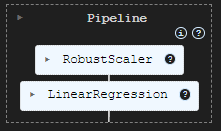
We then wrap a Linear Regression model in a Pipeline and train it.
pipe_model = Pipeline([
    ("scaler", RobustScaler()),
    ("LR", LinearRegression())
])

pipe_model.fit(X_train, y_train) # Training a Linear regression model
Outputs
To evaluate the model we have, I decided to predict the target based on the training and testing data, added this information into a Pandas Dataframe, and then plotted the outcome using Seaborn and Matplotlib.
# Preparing the data for plotting

train_pred = pipe_model.predict(X_train)
test_pred = pipe_model.predict(X_test)


train_data = pd.DataFrame({
    'Index': range(len(y_train)),
    'True Values': y_train,
    'Predicted Values': train_pred,
    'Set': 'Train'
})

test_data = pd.DataFrame({
    'Index': range(len(y_test)),
    'True Values': y_test,
    'Predicted Values': test_pred,
    'Set': 'Test'
})

# figure size 750x1000 pixels
fig, axes = plt.subplots(2, 1, figsize=(7.5, 10), sharex=False)

# Plot Train Data
sns.lineplot(ax=axes[0], data=train_data, x='Index', y='True Values', label='True Values', color='blue')
sns.lineplot(ax=axes[0], data=train_data, x='Index', y='Predicted Values', label='Predicted Values', color='orange')
axes[0].set_title(f'Train Set: True vs Predicted Values | Acc = {r2_score(y_train, train_pred)}', fontsize=14)
axes[0].set_ylabel('Values', fontsize=12)
axes[0].legend()

# Plot Test Data
sns.lineplot(ax=axes[1], data=test_data, x='Index', y='True Values', label='True Values', color='blue')
sns.lineplot(ax=axes[1], data=test_data, x='Index', y='Predicted Values', label='Predicted Values', color='orange')
axes[1].set_title(f'Test Set: True vs Predicted Values | Acc = {r2_score(y_test, test_pred)}', fontsize=14)
axes[1].set_xlabel('Index', fontsize=12)
axes[1].set_ylabel('Values', fontsize=12)
axes[1].legend()

# Final adjustments
plt.tight_layout()
plt.show()
Outputs
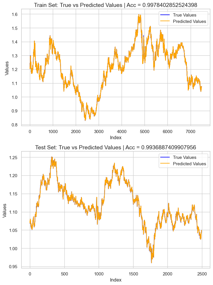
The result is an overfit model with approximately 0.99 r2 score. This is not a good sign of the well-being of the model. Let's inspect the feature importance to observe which features were affecting the model in a positively, those with a bad influence on the model will be removed when detected.
# Extract the linear regression model from the pipeline
lr_model = pipe_model.named_steps['LR']

# Get feature importance (coefficients)
feature_importance = pd.Series(lr_model.coef_, index=X_train.columns)

# Sort feature importance
feature_importance = feature_importance.sort_values(ascending=False)

print(feature_importance)
Outputs
macd main            266.706747
close                  0.093652
open                   0.093435
Avg price              0.042505
close lag_1            0.006972
close lag_3            0.003645
bb_upper               0.001423
close lag_5            0.001415
bb_middle              0.000766
high_low               0.000201
bb_lower               0.000087
var close 5 days      -0.000179
ATR 14                -0.000185
close pct_change      -0.001046
close lag_4           -0.002636
close lag_2           -0.003881
open_close            -0.004705
high                  -0.008575
low                   -0.008663
macd histogram     -5504.010453
macd signal        -5518.035201
dtype: float64
The most informative feature was the macd main, while the macd histogram and macd signal were the least informative variables to the model. Let us drop all the values with negative feature importance, re-train the model then observe the accuracy again.
X = df.drop(columns=[
    "future_close", # drop the target veriable from the independent variables matrix
    "var close 5 days",
    "ATR 14",
    "close pct_change",
    "close lag_4",
    "close lag_2",
    "open_close",
    "high",
    "low",
    "macd histogram",
    "macd signal"
])
pipe_model = Pipeline([
    ("scaler", MinMaxScaler()),
    ("LR", LinearRegression())
])

pipe_model.fit(X_train, y_train)
The accuracy of the re-trained model was very similar to the prior model, The model was still an overfit one. That's fine for now, let's proceed to export the model into ONNX format.
Deploying a Machine Learning Model in MQL5
Inside our Expert Advisor (EA), we start by adding the model as a resource so that it can be compiled with the program.
File: LR model Test.mq5
#resource "\\Files\\EURUSD.dailytf.model.onnx" as uchar lr_onnx[]
We import all the necessary libraries, The Pandas library, ta-lib (for indicators), and Linear Regression (for loading the model).
#include <Linear Regression.mqh>
#include <MALE5\pandas.mqh>
#include <ta-lib.mqh>

CLinearRegression lr;
We initialize the linear regression model in the OnInit function.
int OnInit()
  {
//---

   if (!lr.Init(lr_onnx))
     return INIT_FAILED;

//---
   return(INIT_SUCCEEDED);
  }
The good thing about using this custom Pandas library we have is that, you don't have to start writing code from scratch to collect the data again, we just have to copy the code we used and paste it into the main expert advisor and make tiny modifications to it.
void OnTick()
  {
//---

    CDataFrame df;
    int size = 10000; //We collect this amount of bars for training purposes

    vector open, high, low, close;
    open.CopyRates(Symbol(), PERIOD_D1, COPY_RATES_OPEN,1, size);
    high.CopyRates(Symbol(), PERIOD_D1, COPY_RATES_HIGH,1, size);
    low.CopyRates(Symbol(), PERIOD_D1, COPY_RATES_LOW,1, size);
    close.CopyRates(Symbol(), PERIOD_D1, COPY_RATES_CLOSE,1, size);

    df.Insert("open",open);
    df.Insert("high",high);
    df.Insert("low",low);
    df.Insert("close",close);


    int lags = 5;
    for (int i=1; i<=lags; i++)
      {
         vector lag = df.Shift("close", i);
         df.Insert("close lag_"+string(i), lag);
      }

    vector pct_change = df.Pct_change("close");
    df.Insert("close pct_change", pct_change);

    vector var_5 = df.Rolling("close", 5).Var();
    df.Insert("var close 5 days", var_5);

    df.Insert("open_close",open-close);
    df.Insert("high_low",high-low);

    df.Insert("Avg price",(open+high+low+close)/4);

//---

    BB_res_struct bb = CTrendIndicators::BollingerBands(close,20,0,2.000000); //Calculating the bollinger band indicator

    df.Insert("bb_lower",bb.lower_band); //Inserting lower band values
    df.Insert("bb_middle",bb.middle_band); //Inserting the middle band values
    df.Insert("bb_upper",bb.upper_band); //Inserting the upper band values

    vector atr = COscillatorIndicators::ATR(high,low,close,14);  //Calculating the ATR Indicator

    df.Insert("ATR 14",atr); //Inserting the ATR indicator values

    MACD_res_struct macd = COscillatorIndicators::MACD(close,12,26,9); //MACD indicator applied to the closing price

    df.Insert("macd histogram", macd.histogram); //Inserting the MAC historgram values
    df.Insert("macd main", macd.main); //Inserting the macd main line values
    df.Insert("macd signal", macd.signal);  //Inserting the macd signal line values

    df.Info();
    CDataFrame new_df = df.Dropnan();

    new_df.Head();

    string csv_name = Symbol()+".dailytf.data.csv";
    new_df.ToCSV(csv_name, false, 8);
  }
The modifications include;
Modifying the size of data we want. We no longer need 10000 bars, we just need about 30 bars because the MACD indicator has a period of 26, the Bollinger bands have a period of 20, and the ATR has a period of 14. By giving this a value of 30 we effectively leave some room for calculations.
The OnTick function can be very fluent and explosive sometimes, we don't need to redefine the variables every time a new tick is received.
We don't need to save the data into a CSV file we just need the last row of the Dataframe to be assigned into a vector for plugging into the model.
We can wrap these lines of code into a standalone function to make it easier to work with.
vector GetData(int start_bar=1, int size=30)
 {
    open_.CopyRates(Symbol(), PERIOD_D1, COPY_RATES_OPEN,start_bar, size);
    high_.CopyRates(Symbol(), PERIOD_D1, COPY_RATES_HIGH,start_bar, size);
    low_.CopyRates(Symbol(), PERIOD_D1, COPY_RATES_LOW,start_bar, size);
    close_.CopyRates(Symbol(), PERIOD_D1, COPY_RATES_CLOSE,start_bar, size);

    df_.Insert("open",open_);
    df_.Insert("high",high_);
    df_.Insert("low",low_);
    df_.Insert("close",close_);


    int lags = 5;
    vector lag = {};

    for (int i=1; i<=lags; i++)
      {
         lag = df_.Shift("close", i);
         df_.Insert("close lag_"+string(i), lag);
      }

    pct_change = df_.Pct_change("close");
    df_.Insert("close pct_change", pct_change);

    var_5 = df_.Rolling("close", 5).Var();
    df_.Insert("var close 5 days", var_5);

    df_.Insert("open_close",open_-close_);
    df_.Insert("high_low",high_-low_);

    df_.Insert("Avg price",(open_+high_+low_+close_)/4);

//---

    BB_res_struct bb = CTrendIndicators::BollingerBands(close_,20,0,2.000000); //Calculating the bollinger band indicator

    df_.Insert("bb_lower",bb.lower_band); //Inserting lower band values
    df_.Insert("bb_middle",bb.middle_band); //Inserting the middle band values
    df_.Insert("bb_upper",bb.upper_band); //Inserting the upper band values

    atr = COscillatorIndicators::ATR(high_,low_,close_,14);  //Calculating the ATR Indicator

    df_.Insert("ATR 14",atr); //Inserting the ATR indicator values

    MACD_res_struct macd = COscillatorIndicators::MACD(close_,12,26,9); //MACD indicator applied to the closing price

    df_.Insert("macd histogram", macd.histogram); //Inserting the MAC historgram values
    df_.Insert("macd main", macd.main); //Inserting the macd main line values
    df_.Insert("macd signal", macd.signal);  //Inserting the macd signal line values


    CDataFrame new_df = df_.Dropnan(); //Drop NaN values
    return new_df.Loc(-1); //return the latest row
 }
This is how we initially collected data for training, some of the features present in this function did not make it to the final model due to various reasons, We had to drop them, similarly to how we dropped them inside the Python script.
vector GetData(int start_bar=1, int size=30)
 {
    open_.CopyRates(Symbol(), PERIOD_D1, COPY_RATES_OPEN,start_bar, size);
    high_.CopyRates(Symbol(), PERIOD_D1, COPY_RATES_HIGH,start_bar, size);
    low_.CopyRates(Symbol(), PERIOD_D1, COPY_RATES_LOW,start_bar, size);
    close_.CopyRates(Symbol(), PERIOD_D1, COPY_RATES_CLOSE,start_bar, size);

    df_.Insert("open",open_);
    df_.Insert("high",high_);
    df_.Insert("low",low_);
    df_.Insert("close",close_);


    int lags = 5;
    vector lag = {};

    for (int i=1; i<=lags; i++)
      {
         lag = df_.Shift("close", i);
         df_.Insert("close lag_"+string(i), lag);
      }

    pct_change = df_.Pct_change("close");
    df_.Insert("close pct_change", pct_change);

    var_5 = df_.Rolling("close", 5).Var();
    df_.Insert("var close 5 days", var_5);

    df_.Insert("open_close",open_-close_);
    df_.Insert("high_low",high_-low_);

    df_.Insert("Avg price",(open_+high_+low_+close_)/4);

//---

    BB_res_struct bb = CTrendIndicators::BollingerBands(close_,20,0,2.000000); //Calculating the bollinger band indicator

    df_.Insert("bb_lower",bb.lower_band); //Inserting lower band values
    df_.Insert("bb_middle",bb.middle_band); //Inserting the middle band values
    df_.Insert("bb_upper",bb.upper_band); //Inserting the upper band values

    atr = COscillatorIndicators::ATR(high_,low_,close_,14);  //Calculating the ATR Indicator

    df_.Insert("ATR 14",atr); //Inserting the ATR indicator values

    MACD_res_struct macd = COscillatorIndicators::MACD(close_,12,26,9); //MACD indicator applied to the closing price

    df_.Insert("macd histogram", macd.histogram); //Inserting the MAC historgram values
    df_.Insert("macd main", macd.main); //Inserting the macd main line values
    df_.Insert("macd signal", macd.signal);  //Inserting the macd signal line values


    df_ = df_.Drop(
       //"future_close",
       "var close 5 days,"+
       "ATR 14,"+
       "close pct_change,"+
       "close lag_4,"+
       "close lag_2,"+
       "open_close,"+
       "high,"+
       "low,"+
       "macd histogram,"+
       "macd signal"
    );

    CDataFrame new_df = df_.Dropnan();

    return new_df.Loc(-1); //return the latest row
 }
Instead of dropping the columns like in the above function, It is wise to remove the code used to produce them in the first place, this could reduce unnecessary computations which may slow the program when there are a lot of features to calculate just so they can be dropped shortly.
We are going to stick with the Drop method for now.
After calling the Head() method to see what's on the Dataframe, below was the outcome:
PM      0       15:45:36.543    LR model Test (EURUSD,H1)       CDataFrame::Dropnan completed. Rows dropped: 25/30
HI      0       15:45:36.543    LR model Test (EURUSD,H1)       | open           | close          | close lag_1     | close lag_3     | close lag_5     | high_low       | Avg price      | bb_lower       | bb_middle      | bb_upper       | macd main      |
GK      0       15:45:36.543    LR model Test (EURUSD,H1)       | 1.04057000     | 1.04079000     | 1.04057000      | 1.02806000      | 1.03015000      | 0.00575000     | 1.04176750     | 1.02125891     | 1.03177350     | 1.04228809     | 0.00028705     |
QI      0       15:45:36.543    LR model Test (EURUSD,H1)       | 1.04079000     | 1.04159000     | 1.04079000      | 1.04211000      | 1.02696000      | 0.00661000     | 1.04084750     | 1.02081967     | 1.03210400     | 1.04338833     | 0.00085370     |
PL      0       15:45:36.543    LR model Test (EURUSD,H1)       | 1.04158000     | 1.04956000     | 1.04159000      | 1.04057000      | 1.02806000      | 0.01099000     | 1.04611250     | 1.01924805     | 1.03282750     | 1.04640695     | 0.00192371     |
JR      0       15:45:36.543    LR model Test (EURUSD,H1)       | 1.04795000     | 1.04675000     | 1.04956000      | 1.04079000      | 1.04211000      | 0.00204000     | 1.04743000     | 1.01927184     | 1.03382650     | 1.04838116     | 0.00251595     |
CP      0       15:45:36.543    LR model Test (EURUSD,H1)       | 1.04675000     | 1.04370000     | 1.04675000      | 1.04159000      | 1.04057000      | 0.01049000     | 1.04664500     | 1.01938012     | 1.03447300     | 1.04956588     | 0.00270798     |
CH      0       15:45:36.543    LR model Test (EURUSD,H1)       (5x11)
We have 11 features, The same number of features can be seen on the model.
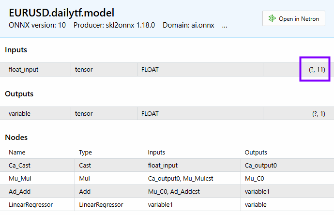
Below is how we can get the final model's predictions.
void OnTick()
  {
     vector x = GetData();
     Comment("Predicted close: ", lr.predict(x));
  }
It is not smart to perform all the data collection and model calculations on every tick, we need to calculate them at the opening of a new bar on the chart.
void OnTick()
  {
     if (isNewBar())
       {
           vector x = GetData();
           Comment("Predicted close: ", lr.predict(x));
       }
  }
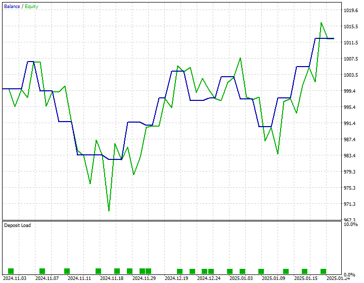
I developed a simple strategy to place a buy trade whenever the predicted closing price is above the current bid price and place a sell trade whenever the predicted closing price is below the current ask price.
Below is the strategy tester outcome from 01 November 2024 to January 25, 2025.
Conclusion
It is now easy to import sophisticated AI models into MQL5 and use them in MetaTrader 5 like nothing, It is still not easy to keep your model in sync with the data structure similar to the one used for training. In this article, I introduced a custom class named CDataframe to aid us when dealing with two-dimensional data in an environment that feels like the one in Pandas library which is very familiar to the machine learning community and data scientists coming from a Python background.
It is my hope the Pandas library in MQL5 will be of good use and make our lives much easier when dealing with complex AI data in MQL5.
Best regards.
Stay tuned and contribute to machine learning algorithms development for MQL5 language in this GitHub repository.
Attachments Table
| Filename | Description/Usage |
|---|---|
| Experts\LR model Test.mq5 | An Expert advisor for deploying the final linear regression model. |
| Include\Linear Regression.mqh | A library containing all the code for loading a Linear regression model in ONNX format. |
| Include\pandas.mqh | Consists all the custom Pandas methods for working with data in a Dataframe class. |
| Scripts\pandas test.mq5 | A script responsible for collecting the data for ML training purposes. |
| Python\main.ipynb | A jupyter notebook file with all the code for training a linear regression model used in this article. |
| Files\ | This folder consists of a linear regression model in ONNX models and CSV files for AI models training purposes. |
Warning: All rights to these materials are reserved by MetaQuotes Ltd. Copying or reprinting of these materials in whole or in part is prohibited.
This article was written by a user of the site and reflects their personal views. MetaQuotes Ltd is not responsible for the accuracy of the information presented, nor for any consequences resulting from the use of the solutions, strategies or recommendations described.

- Free trading apps
- Over 8,000 signals for copying
- Economic news for exploring financial markets
You agree to website policy and terms of use