

First Fractal Breakout — Intraday Strategy, Expert Advisor and Backtesting
 2 047
2 047
 0
0

Introduction
The First Fractal Breakout is an intraday trading strategy designed to capture the most decisive moves of the active trading session of an instrument. It is a session-bound strategy that utilizes the first Bill Williams market fractals to determine the breakout limits. Standard opening range breakout (ORB) strategies often use an arbitrary time window or prior-session levels. This strategy instead assumes that fractals record the market's microstructure. This distinguishes the system with key advantages:
- Market Structure Driven: The breakout limits are defined by fractals, which are five-bar pivots formed by the actual price structure and are not time-driven like ORB.
- Adaptive Boundaries: The breakout levels vary in width alongside market volatility. A quiet opening produces a tight fractal range, while a volatile opening expands the range. The strategy dynamically adapts to the day's trading activity instead of forcing a fixed time window.
- Bidirectional Execution: The strategy allows for one long and one short trade attempt per session. It can capture wide, significant two-way swings in volatile conditions.
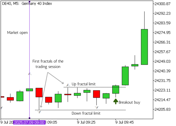
First Fractal Breakout Strategy
In this article, we will develop the First Fractal Breakout trading strategy around the following core features:
- Instrument-specific trading session, aligning activity with the hours when the instrument's volatility is most reliable.
- Self-drawn breakout levels, obtained from intraday fractals, independent of trader subjectivity.
- Bidirectional trading, aimed at capturing one long and short breakout move during the day.
- Volatility-based stop-losses to dynamically account for active trading days.
- Position sizing based on percentage risk to keep risk consistent across volatility regimes and automatically scale with accrued balance.
- Fixed reward-to-risk ratio, optimizable through backtesting.
- Guaranteed flat close at session end.
- No overnight risk and swap funding costs.
We will build the strategy from first principles and use the DAX (European session) as the working example. The article will walk through the trading premise, session bounds definition, parameter selection, strategy algorithm, and expert advisor code implementation. We will backtest the system using 100% quality tick data over a broad parameter space and analyze the results to determine the efficacy of the premise. Ultimately, we will show that using fractals to determine breakout limits offers a practical and viable framework for intraday trading. Dates use YYYY-MM-DD format. Times use Moscow Standard Time (MSK, UTC+3). Prices are in USD.
Trading Premise
The core premise of this strategy is that fractals are the market's own record of its microstructure, particularly a completed swing. A Bill Williams fractal is defined as a pattern of five consecutive candlesticks where the middle candle establishes a local extreme relative to the surrounding two candles on each side. Depending on the direction, we can categorize them as follows:
- Up Fractal: Formed when the middle candle (bar) has the highest high among the five, marked by an arrow above the high.
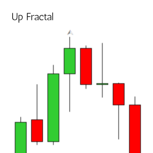
Up Fractal
-
Down Fractal: Formed when the middle candle (bar) has the lowest low among the five, marked by an arrow below the low.
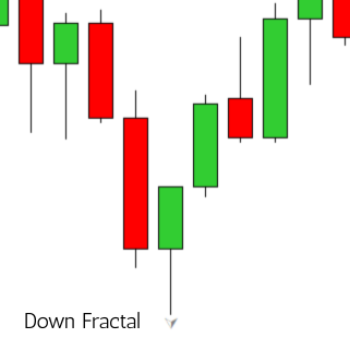
Down Fractal
Fractals are part of the standard MQL5 indicator set and can be called using the iFractals function. The first up fractal and first down fractal to form after the session opens mark the first confirmed swing high and swing low of the day. Together they define a natural, price-drawn range, which forms the levels for breakout trades.
There is a catch, however, when working with fractals. Because a fractal needs two bars to close after the central bar to confirm it, a fractal is always identified with a two-bar delay. Fractals within two bars of the current bar are susceptible to repainting. This matters in the selection of the intraday candle timeframe over which the fractals need to be identified. We will need at least three bars to define a breakout limit. For this strategy we will be using the M5 timeframe. The M1 timeframe can lead to very tight ranges in the first few minutes caused by high-volume noise, leading to quick breakouts that are not representative of the day's trading activity. With the M5 timeframe, we will need to wait at least 15 minutes into the session, which is sufficient time for the opening noise to subside.
The trading premise favors sessions with an initial consolidation followed by directional expansion, which is a common intraday pattern captured by breakout strategies. However, in strong trending markets without fractal formations due to a lack of reversals, the strategy could remain flat.
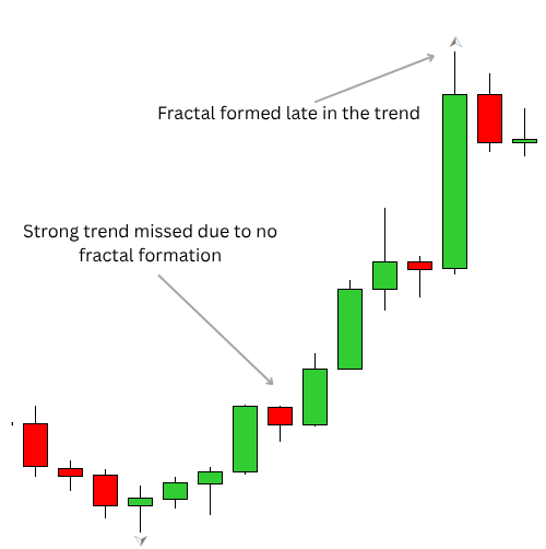
Fractals in strongly trending markets
To work around this inherent limitation of fractal breakouts, we need to be strategic in selecting our session bounds. Runaway directional moves are more frequent in markets with active stock exchange operations. For the DAX, this corresponds to the active Xetra session from 10:00 to 18:30, during which core cash trading occurs. To maximize our chances of capturing trending moves, we should expand our session bounds slightly into the extended sessions. For the DAX, we will start at 9:00 and close all positions at 18:45. Alternatively, session bounds based on volume analysis could also be utilized.
Parameter Selection
With the fractal limits forming the candidate entry points, we hold that the market establishes its breakout direction once a limit is broken. This gives us a maximum of two trade attempts per day. Capping exposure at one attempt per direction aligns with the premise of the first fractals forming the opening range and avoids whipsaws caused by repeated entries with no additional information.
The next parameters to determine are the trade size, stop-loss distance, and the reward-to-risk ratio. For this strategy, we will use the fixed percentage risk per trade. The advantages to using a percent-based risk system are:
- The lot sizes auto-scale with the accrued balance. It serves as capital preservation during a losing streak and compounding during a winning streak.
- It offers a realistic view of drawdown expectations in backtests and optimizations.
- One trade per side explicitly limits the maximum daily account exposure to twice the risk percentage.
We will opt for a dynamic stop-loss distance that adapts to market volatility. We can measure volatility using the Average True Range (ATR). For intraday moves, the D1 ATR gives us a proportional estimate of the potential range of price moves. Since the ATR also includes overnight moves, we can treat it as a theoretical upper bound and use a fraction of the D1 ATR as the stop-loss distance. To determine the optimal fraction, we will run an optimization over a range of percentages of the D1 ATR.
To determine the take-profit levels, we will need the reward-to-risk ratio or the take-profit multiplier the strategy is targeting. This too could be obtained by an optimization over a range of values over the daily timeframe. Together, the ATR percentage and the take-profit multiplier form the two optimizable strategy parameters that define the strategy. While it is also possible to optimize the session bounds and the risk per trade along with the strategy parameters, it would make the backtests vulnerable to overfitting and lead to false conclusions. Limiting the optimizations to two parameters is in line with best algorithmic trading practices.
Strategy
We can now define the strategy algorithm:
- Check if the market is open and at least 15 minutes from the start time have elapsed.
- If the up fractal limit is not set, obtain the up fractal value of the third M5 bar from the current forming bar. If it is a confirmed up fractal, set it as the up fractal limit.
- If the down fractal limit is not set, obtain the down fractal value of the third M5 bar from the current forming bar. If it is a confirmed down fractal, set it as the down fractal limit.
- If the up fractal limit is set and a buy position is not opened for the day, check if the current bid price (fractals are based on the bid price) has broken the up fractal limit. If yes, open a market buy trade at the user-input risk percentage per trade lot size, ATR percentage stop-loss distance, and take-profit multiplier. Mark the buy trade as done.
- If the down fractal limit is set and a sell position is not opened for the day, check if the current bid price has broken the down fractal limit. If yes, open a market sell trade at the user-input risk percentage per trade lot size, ATR percentage stop-loss distance, and take-profit multiplier. Mark the sell trade as done.
- Repeat steps 1 to 5 every tick until the session closes. When the end time is reached, close all remaining open positions and reset all the fractal limits and trade flags for the next trading day. Mark the session as closed until the next start time.
Expert Advisor
Let us automate the strategy in an MQL5 Expert Advisor (EA). Fractalstruct is a lightweight wrapper around the fractal value and time with a bool field to represent if the fractal limit is set. FractalTypeenum denotes the type of fractals.
enum FractalType
  {
   fractal_high = 0,
   fractal_low  = 1
  };

struct Fractal
  {
   bool     isSet;
   double   value;
   datetime time;

   Fractal(bool IsSet=false, double Value=0, datetime Time=0):
      isSet(IsSet),
      value(Value),
      time(Time) {}
  };
The handles for the ATR and fractal indicators are declared as global variables along with the intraday FractalTimeFrame and AtrTimeframe. The FractalShift value denotes the shift from the current forming FractalTimeFrame bar in the iFractals function. As explained in the Trading Premise section, we query the fractal buffer at shift 3 to ensure the fractal is fully confirmed. Since we only need to retrieve a single value of the indicators, we define wrappers to the CopyBuffer function. We also define the master CTrade object, Trade for easy access to trade functions.
int AtrHandle;
int FractalHandle;

CTrade Trade;

ENUM_TIMEFRAMES FractalTimeframe = PERIOD_M5;
ENUM_TIMEFRAMES AtrTimeframe     = PERIOD_D1;
int             FractalShift     = 3;

//+------------------------------------------------------------------+
//| Returns the value of fractal indicator                           |
//+------------------------------------------------------------------+
double GetFractal(const int &fractalHandle, FractalType fractalType, int shift)
  {
   double fractal[];
   if(CopyBuffer(fractalHandle,(int) fractalType,shift,1,fractal) == -1)
      return EMPTY_VALUE;
   return fractal[0];
  }

//+------------------------------------------------------------------+
//| Returns the value of ATR indicator                               |
//+------------------------------------------------------------------+
double GetATR(const int &atrHandle)
  {
   double atr[];
   if(CopyBuffer(atrHandle,0,1,1,atr) == -1)
      return EMPTY_VALUE;
   return atr[0];
  }
The GetStrategyFractal function constructs the Fractal from the indicator values. For valid fractal values, we cross-check the time stamp using iTime against the input startTime to confirm that the fractal is formed after the session start.
//+--------------------------------------------------------------------+
//| Returns a Fractal type constructed from the indicator fractal value|
//+--------------------------------------------------------------------+
Fractal GetStrategyFractal(const int &fractalHandle, FractalType fractalType, int shift, ENUM_TIMEFRAMES timeframe, datetime startTime)
  {
   double fractalValue = GetFractal(FractalHandle, fractalType, shift);
   if(fractalValue != EMPTY_VALUE)
     {
      datetime time = iTime(Symbol(), timeframe, shift);
      if(time >= startTime)
        {
         return Fractal(true, fractalValue, time);
        }
     }
   return Fractal();
  }
Confirmed fractals are updated once per bar; we need not check them on every tick. We will maintain the state of the last forming FractalTimeFrame bar in gblLastFractalBar and update it in the IsNewFractalBar check function.
datetime gblLastFractalBar;

//+------------------------------------------------------------------+
//| Returns if new bar of the fractal timeframe is formed            |
//+------------------------------------------------------------------+
bool IsNewFractalBar()
  {
   datetime curTime = iTime(Symbol(), FractalTimeframe, 0);
   if(curTime != gblLastFractalBar)
     {
      gblLastFractalBar = curTime;
      return true;
     }
   return false;
  }
The inputs to the EA are defined as shown below. InpStartHour, InpStartMin, InpEndHour, and InpEndMin together define the session bounds. The ATR period is configurable through InpAtrPeriod. InpAtrPercent and InpTpMultiplier are the strategy parameters, and InpRiskPercentPerTrade is the percentage risk per trade. InpShowObjects toggles visual objects, and InpMagicNumber helps to uniquely identify trades placed by the EA.
input group    "Start Time"
input int      InpStartHour               = 9;        // Start Hour (0 - 23)
input int      InpStartMin                = 0;        // Start Min (0 - 59)
input group    "End Time"
input int      InpEndHour                 = 18;       // End Hour (0 - 23)
input int      InpEndMin                  = 45;       // End Min (0 - 59)
input group    "Trade Parameters"
input double   InpRiskPercentPerTrade     = 1;        // Risk Percent Per Trade
input int      InpAtrPeriod               = 14;       // ATR Period
input group    "Strategy Parameters"
input double   InpAtrPercent              = 15;       // ATR Percentage
input double   InpTpMultiplier            = 10;       // TP Multiplier
input group    "Visual Objects"
input bool     InpShowObjects             = true;     // Draw Visual Objects
input group    "Expert Identification"
input ulong    InpMagicNumber             = 12345;    // Magic Number
StartMinOffset defines how many minutes after session start the EA begins searching for confirmed fractals. This value needs to be at least FractalTimeframe * FractalShift to ensure only fractal values after the session start are considered. We will set this to 15 minutes. The SessionTimestruct holds the start, strategyStart,and end times for the trading day with an isSessionSet flag to indicate if values are populated. We will maintain the session state globally in gblSession and set it for the current day in the SetSessionTimes function using the methods of the CDateTime class and the EA inputs. The DayInc method will accurately add a day to the closing time when the session crosses over midnight.
int StartMinOffset = 15;

SessionTime gblSession;

//+------------------------------------------------------------------+
//| Sets start, strategy and end times for the current trading day   |
//+------------------------------------------------------------------+
void SetSessionTimes()
  {
   CDateTime start;
   CDateTime end;
   CDateTime strategy;

   start.Date(TimeCurrent());
   start.Hour(InpStartHour);
   start.Min(InpStartMin);
   start.Sec(0);

   strategy.DateTime(start.DateTime());
   strategy.MinInc(StartMinOffset);

   end.Date(TimeCurrent());
   end.Hour(InpEndHour);
   end.Min(InpEndMin);
   end.Sec(0);

//--- Increment ending date by 1 day if closing crosses over midnight
   if((InpEndHour < InpStartHour) ||
      ((InpStartHour == InpEndHour) && (InpEndMin <= InpStartMin)))
     {
      end.DayInc(1);
     }

   gblSession.start           = start.DateTime();
   gblSession.strategyStart   = strategy.DateTime();
   gblSession.end             = end.DateTime();
   gblSession.isSessionSet    = true;
  }
The DirectionStats structure maintains a cumulative count of the trades by their closing reason and their gross profit and loss along a single trading direction. The ExpertStats structure contains one DirectionStats field each for buy and sell trades. By categorizing trades this way, we can analyze the source of trading profits by the closing reason. We will maintain the cumulative stats in the gblStats instance throughout the lifecycle of the EA and print it using the PrintStats function at deinitialization.
ExpertStats    gblStats;

struct DirectionStats
  {
   int slCount;
   int tpCount;
   int closeProfitCount;
   int closeLossCount;
   double slGross;
   double tpGross;
   double closeProfitGross;
   double closeLossGross;

   DirectionStats(int SlCount=0, int TpCount=0, int CloseProfitCount=0, int CloseLossCount=0, double SlGross=0, double TpGross=0, double CloseProfitGross=0, double CloseLossGross=0):
      slCount(SlCount),
      tpCount(TpCount),
      closeProfitCount(CloseProfitCount),
      closeLossCount(CloseLossCount),
      slGross(SlGross),
      tpGross(TpGross),
      closeProfitGross(CloseProfitGross),
      closeLossGross(CloseLossGross) {}
  };

struct ExpertStats
  {
   DirectionStats buy;
   DirectionStats sell;

   ExpertStats():
      buy(DirectionStats()),
      sell(DirectionStats()) {}
  };

//+------------------------------------------------------------------+
//| Prints the strategy stats during the expert lifetime             |
//+------------------------------------------------------------------+
void PrintStats()
  {
   Print("=== Summary Stats ==="
         "\n--- Long ---",
         "\nSl count: ",            gblStats.buy.slCount,
         "\nSl gross: ",            gblStats.buy.slGross,
         "\nTp count: ",            gblStats.buy.tpCount,
         "\nTp gross: ",            gblStats.buy.tpGross,
         "\nClose profit count: ",  gblStats.buy.closeProfitCount,
         "\nClose profit gross: ",  gblStats.buy.closeProfitGross,
         "\nClose loss count: ",    gblStats.buy.closeLossCount,
         "\nClose loss gross: ",    gblStats.buy.closeLossGross,
         "\n--- Short ---",
         "\nSl count: ",            gblStats.sell.slCount,
         "\nSl gross: ",            gblStats.sell.slGross,
         "\nTp count: ",            gblStats.sell.tpCount,
         "\nTp gross: ",            gblStats.sell.tpGross,
         "\nClose profit count: ",  gblStats.sell.closeProfitCount,
         "\nClose profit gross: ",  gblStats.sell.closeProfitGross,
         "\nClose loss count: ",    gblStats.sell.closeLossCount,
         "\nClose loss gross: ",    gblStats.sell.closeLossGross,
         "\n--- Total ---",
         "\nSl count: ",            gblStats.sell.slCount + gblStats.buy.slCount,
         "\nSl gross: ",            gblStats.sell.slGross + gblStats.buy.slGross,
         "\nTp count: ",            gblStats.sell.tpCount + gblStats.buy.tpCount,
         "\nTp gross: ",            gblStats.sell.tpGross + gblStats.buy.tpGross,
         "\nClose profit count: ",  gblStats.sell.closeProfitCount + gblStats.buy.closeProfitCount,
         "\nClose profit gross: ",  gblStats.sell.closeProfitGross + gblStats.buy.closeProfitGross,
         "\nClose loss count: ",    gblStats.sell.closeLossCount   + gblStats.buy.closeLossCount,
         "\nClose loss gross: ",    gblStats.sell.closeLossGross   + gblStats.buy.closeLossGross);
  }
The visual objects consist of the session bounds and fractal limits. We will prefix all objects with ObjPrefix to facilitate easier cleanup at deinitialization. As the objects need to be drawn for every session, we will derive names from the string representation of the session bounds and append suffixes based on object type to satisfy uniqueness. The VisualObjects structure contains flags to keep track of the objects drawn. We will maintain the state of the visuals drawn using the DrawVisualObjects function in the gblVisuals instance.
struct VisualObjects
  {
   bool isSession;
   bool isUpFractal;
   bool isDnFractal;

   VisualObjects(bool IsSession=false, bool IsUpFractal=false, bool IsDnFractal=false):
      isSession(IsSession),
      isUpFractal(IsUpFractal),
      isDnFractal(IsDnFractal) {}
  };

string ObjPrefix        = "fractal_breakout_";
string StartSuffix      = "_start";
string EndSuffix        = "_end";
string UpFractalSuffix  = "_up_fractal";
string DnFractalSuffix  = "_dn_fractal";
string StartLabel       = "Session Start";
string EndLabel         = "Session Close";
string UpFractalLabel   = "Up Fractal Limit";
string DnFractalLabel   = "Dn Fractal Limit";
color  StartColor       = clrCyan;
color  EndColor         = clrViolet;
color  UpFractalColor   = clrAzure;
color  DnFractalColor   = clrBlanchedAlmond;

VisualObjects  gblVisuals;

//+------------------------------------------------------------------+
//| Draws objects for strategy visualization                         |
//+------------------------------------------------------------------+
void DrawVisualObjects(const SessionTime &session, const Fractal &up, const Fractal &dn, VisualObjects &visuals)
  {
   long chartId   = ChartID();
   int  subWindow = 0;
   if(session.isSessionSet && !visuals.isSession)
     {
      string startName = ObjPrefix + TimeToString(session.start) + StartSuffix;
      ObjectCreate(chartId, startName, OBJ_VLINE, subWindow, session.start, 0);
      ObjectSetInteger(chartId, startName, OBJPROP_COLOR, StartColor);
      ObjectSetString(chartId, startName, OBJPROP_TEXT, StartLabel);

      string endName = ObjPrefix + TimeToString(session.end) + EndSuffix;
      ObjectCreate(chartId, endName, OBJ_VLINE, subWindow, session.end, 0);
      ObjectSetInteger(chartId, endName, OBJPROP_COLOR, EndColor);
      ObjectSetString(chartId, endName, OBJPROP_TEXT, EndLabel);

      visuals.isSession = true;
     }

   if(up.isSet && !visuals.isUpFractal)
     {
      string upFractalName = ObjPrefix + TimeToString(session.start) + UpFractalSuffix;
      ObjectCreate(chartId, upFractalName, OBJ_TREND, subWindow, up.time, up.value, session.end, up.value);
      ObjectSetInteger(chartId, upFractalName, OBJPROP_STYLE, STYLE_DASH);
      ObjectSetInteger(chartId, upFractalName, OBJPROP_COLOR, UpFractalColor);
      ObjectSetString(chartId, upFractalName, OBJPROP_TEXT, UpFractalLabel);

      visuals.isUpFractal = true;
     }

   if(dn.isSet && !visuals.isDnFractal)
     {
      string dnFractalName = ObjPrefix + TimeToString(session.start) + DnFractalSuffix;
      ObjectCreate(chartId, dnFractalName, OBJ_TREND, subWindow, dn.time, dn.value, session.end, dn.value);
      ObjectSetInteger(chartId, dnFractalName, OBJPROP_STYLE, STYLE_DASH);
      ObjectSetInteger(chartId, dnFractalName, OBJPROP_COLOR, DnFractalColor);
      ObjectSetString(chartId, dnFractalName, OBJPROP_TEXT, DnFractalLabel);

      visuals.isDnFractal = true;
     }
  }
The states of the up and down fractal limits will be held in gblUpFractal and gblDnFractal. Flags gblIsOpen will indicate if the market is open, and gblIsStrategy will indicate if the necessary time for the strategy since the session open has elapsed. Flags gblIsBuyTrade and gblIsSellTrade will denote the status of the buy and sell trade attempt for the day. CDateTime objects gblLastOpenDate will hold the date of the last session open, and gblLastSessionSet will hold the date of the last time the session times were set.
The datetime values of the last buy trade will be held in gblLastBuyTime, and the last sell trade will be held in gblLastSellTime. The InitGlobals function will initialize the values of all the state variables and flags that need to be reset before the start of the next trading session.
Fractal gblUpFractal;
Fractal gblDnFractal;

bool gblIsOpen;
bool gblIsStrategy;
bool gblIsBuyTrade;
bool gblIsSellTrade;

CDateTime gblLastOpenDate;
CDateTime gblLastSessionSet;

datetime gblLastBuyTime;
datetime gblLastSellTime;

//+------------------------------------------------------------------+
//| Initializes global variables                                     |
//+------------------------------------------------------------------+
void InitGlobals()
  {
   gblIsOpen         = false;
   gblIsStrategy     = false;
   gblIsBuyTrade     = false;
   gblIsSellTrade    = false;
   gblUpFractal      = Fractal();
   gblDnFractal      = Fractal();

   if(InpShowObjects)
      gblVisuals = VisualObjects();
  }
The GetLotSize function calculates the lot size for the input risk percent per trade, openPrice, and sl using OrderCalcProfit. The CheckMarginForTrade function checks the account for sufficient free margin to open the trade for a given lot size using OrderCalcMargin. The CheckStopsLevel function checks that slDist exceeds the minimum stop distance and CheckFreezeLevel checks that dist exceeds the broker freeze level.
//+------------------------------------------------------------------+
//| Returns trade lot size for strategy risk percentage              |
//+------------------------------------------------------------------+
double GetLotSize(double openPrice, double sl, ENUM_ORDER_TYPE orderType)
  {
   double minVol  = SymbolInfoDouble(Symbol(), SYMBOL_VOLUME_MIN);
   double maxVol  = SymbolInfoDouble(Symbol(), SYMBOL_VOLUME_MAX);
   double volStep = SymbolInfoDouble(Symbol(), SYMBOL_VOLUME_STEP);
   double profit  = 0;
   if(!OrderCalcProfit(orderType, Symbol(), minVol, openPrice, sl, profit))
     {
      Print("Failed to calculate lot size: ", GetLastError());
      return 0;
     }

   double lossPerMinVol = MathAbs(profit);
   double risk          = AccountInfoDouble(ACCOUNT_BALANCE) * InpRiskPercentPerTrade / 100;
   double lots          = MathFloor((risk / lossPerMinVol * minVol) / volStep) * volStep;

   if(lots < minVol)
      return 0;
   if(lots > maxVol)
      return maxVol;
   return lots;
  }

//+------------------------------------------------------------------+
//| Checks if sufficient free margin is available to initiate trade  |
//+------------------------------------------------------------------+
bool CheckMarginForTrade(double openPrice, double lots, ENUM_ORDER_TYPE orderType)
  {
   double freeMargin = AccountInfoDouble(ACCOUNT_MARGIN_FREE);
   double reqMargin;
   if(!OrderCalcMargin(orderType, Symbol(), lots, openPrice, reqMargin))
     {
      Print("Failed to calculate position margin: ", GetLastError());
      return false;
     }

   if(reqMargin > freeMargin)
     {
      Print("Insufficient funds");
      return false;
     }
   return true;
  }

//+------------------------------------------------------------------+
//| Checks for broker stop levels                                    |
//+------------------------------------------------------------------+
bool CheckStopsLevel(double slDist)
  {
   int stopsLevel = (int) SymbolInfoInteger(Symbol(), SYMBOL_TRADE_STOPS_LEVEL);
   if(stopsLevel == 0)
      return true;
   return (slDist >= stopsLevel * Point()) && (slDist * InpTpMultiplier >= stopsLevel * Point());
  }

//+------------------------------------------------------------------+
//| Checks for broker freeze levels                                  |
//+------------------------------------------------------------------+
bool CheckFreezeLevel(double dist)
  {
   int freezeLevel = (int) SymbolInfoInteger(Symbol(), SYMBOL_TRADE_FREEZE_LEVEL);
   if(freezeLevel == 0)
      return true;
   return dist >= freezeLevel * Point();
  }
The OpenTrade function opens a trade along the posType direction with the price details passed by the MqlTick structure, curTick, after the necessary trading checks. Buy trades are executed on the ask price of the tick for immediate market execution even though the breakout is triggered by the bid price. This can lead to an execution price that differs from the breakout level based on the spread. The slDist is obtained from the InpAtrPercent and GetATR function.
The tp is calculated from slDist and InpTpMultiplier. The sl is calculated by adding or subtracting slDist from the execution price depending on the trade direction. The lot size is obtained from the GetLotSize function, and the trades are executed using the trade methods of the CTrade class. Trade execution results are determined from the return values of the trade methods of the CTrade class and the ResultRetcode. The OpenTrade function returns true on successful trade execution and false otherwise.
//+------------------------------------------------------------------+
//| Opens trade of given position type and tick structure            |
//+------------------------------------------------------------------+
bool OpenTrade(ENUM_POSITION_TYPE posType, MqlTick &curTick)
  {
   double atr = GetATR(AtrHandle);
   if(atr == EMPTY_VALUE)
     {
      Print("Could not read ATR value");
      return false;
     }

   double slDist = InpAtrPercent / 100 * atr;
   if(!CheckStopsLevel(slDist))
      return false;

   switch(posType)
     {
      case POSITION_TYPE_BUY:
        {
         double sl = curTick.ask - slDist;
         double tp = curTick.ask + InpTpMultiplier * slDist;
         if(!CheckFreezeLevel(tp - curTick.bid) || !CheckFreezeLevel(curTick.bid - sl))
            return false;

         double lots = GetLotSize(curTick.ask, sl, ORDER_TYPE_BUY);
         if(lots == 0)
            return false;

         if(!CheckMarginForTrade(curTick.ask, lots, ORDER_TYPE_BUY))
            return false;

         if(!Trade.Buy(lots, Symbol(), curTick.ask, sl, tp))
           {
            Print("Failed to open position: ", Trade.ResultRetcodeDescription());
            return false;
           }
         break;
        }

      case POSITION_TYPE_SELL:
        {
         double sl = curTick.bid + slDist;
         double tp = curTick.bid - InpTpMultiplier * slDist;
         if(!CheckFreezeLevel(curTick.ask - tp) || !CheckFreezeLevel(sl - curTick.ask))
            return false;

         double lots = GetLotSize(curTick.bid, sl, ORDER_TYPE_SELL);
         if(lots == 0)
            return false;

         if(!CheckMarginForTrade(curTick.bid, lots, ORDER_TYPE_SELL))
            return false;

         if(!Trade.Sell(lots, Symbol(), curTick.bid, sl, tp))
           {
            Print("Failed to open position: ", Trade.ResultRetcodeDescription());
            return false;
           }
         break;
        }
     }
   if((Trade.ResultRetcode() != TRADE_RETCODE_DONE))
     {
      Print("Trade opening failed: ", Trade.ResultRetcodeDescription());
      return false;
     }
   return true;
  }
All the remaining open positions of the EA are identified by the position Symbol and InpMagicNumber using the methods of the CPositionInfo class. Positions are closed by the PositionClose method of the CTrade class.
//+------------------------------------------------------------------+
//| Closes all open positions of current symbol and magic number     |
//+------------------------------------------------------------------+
void CloseAllPositions()
  {
   for(int i = PositionsTotal()-1; i >= 0; i--)
     {
      CPositionInfo posInfo;
      if(!posInfo.SelectByIndex(i))
         continue;
      if(posInfo.Symbol() != Symbol() || posInfo.Magic() != InpMagicNumber)
         continue;
      if(!Trade.PositionClose(posInfo.Ticket()))
        {
         Print("Failed to close position: ", posInfo.Ticket(), "Err: ", Trade.ResultRetcodeDescription());
         continue;
        }
      if((Trade.ResultRetcode() != TRADE_RETCODE_DONE))
        {
         Print("Failed to close position: ", posInfo.Ticket(), "Err: ", Trade.ResultRetcodeDescription());
         continue;
        }
     }
  }
The initialization function carries out input validation, obtains indicator handles, and sets the values of the global state and environment variables. The strategy parameter combinations can be set to trigger both long and short trades at the same time; a netting account will cause a net flattening of the strategy by closing an existing position by its opposite side. Therefore, we check the account for hedging mode by the ACCOUNT_MARGIN_MODE property obtained using AccountInfoInteger.
InitGlobals initializes the global state variables and flags for the first trading day. The global variables, gblLastFractalBar and gblStats, that persist beyond trading sessions are also initialized. The chart property CHART_SHOW_OBJECT_DESCR is enabled for object label display.
//+------------------------------------------------------------------+
//| Expert initialization function                                   |
//+------------------------------------------------------------------+
int OnInit()
  {
//--- Check account type
   if(AccountInfoInteger(ACCOUNT_MARGIN_MODE) != ACCOUNT_MARGIN_MODE_RETAIL_HEDGING)
     {
      MessageBox("You need a hedging account for this EA");
      return INIT_AGENT_NOT_SUITABLE;
     }

//--- Input Validation
   if(InpMagicNumber == 0)
     {
      MessageBox("Please enter a Magic Number other than 0");
      return INIT_PARAMETERS_INCORRECT;
     }

   if(InpStartHour < 0 || InpStartHour > 23)
     {
      MessageBox("Please enter start hour between 0 and 23");
      return INIT_PARAMETERS_INCORRECT;
     }

   if(InpStartMin < 0 || InpStartMin > 59)
     {
      MessageBox("Please enter start min between 0 and 59");
      return INIT_PARAMETERS_INCORRECT;
     }

   if(InpEndHour < 0 || InpEndHour > 23)
     {
      MessageBox("Please enter end hour between 0 and 23");
      return INIT_PARAMETERS_INCORRECT;
     }

   if(InpEndMin < 0 || InpEndMin > 59)
     {
      MessageBox("Please enter end min between 0 and 59");
      return INIT_PARAMETERS_INCORRECT;
     }

   if(InpRiskPercentPerTrade <= 0 || InpRiskPercentPerTrade > 100)
     {
      MessageBox("Please enter valid risk percent per trade");
      return INIT_PARAMETERS_INCORRECT;
     }

   if(InpAtrPeriod <= 0)
     {
      MessageBox("Please enter ATR period above 0");
      return INIT_PARAMETERS_INCORRECT;
     }

   if(InpAtrPercent <= 0)
     {
      MessageBox("Please enter ATR percent above 0");
      return INIT_PARAMETERS_INCORRECT;
     }

   if(InpTpMultiplier < 0)
     {
      MessageBox("Please enter TP multiplier greater than or equal to 0");
      return INIT_PARAMETERS_INCORRECT;
     }

   Trade.SetExpertMagicNumber(InpMagicNumber);

//--- Indicator handles
   AtrHandle      = iATR(Symbol(), AtrTimeframe, InpAtrPeriod);
   if(AtrHandle == INVALID_HANDLE)
     {
      MessageBox("Failed to create ATR handle");
      return INIT_FAILED;
     }

   FractalHandle  = iFractals(Symbol(), FractalTimeframe);
   if(FractalHandle == INVALID_HANDLE)
     {
      MessageBox("Failed to create fractal handle");
      return INIT_FAILED;
     }

//--- Initialize global variables
   InitGlobals();
   gblLastFractalBar = iTime(Symbol(), FractalTimeframe, 0);
   gblStats = ExpertStats();

//--- Enable chart property to show object labels
   if(InpShowObjects)
      ChartSetInteger(ChartID(), CHART_SHOW_OBJECT_DESCR, true);
   return INIT_SUCCEEDED;
  }
On deinitialization, the indicator handles are released. The visual chart objects are deleted using ObjectsDeleteAll by identifying them with ObjPrefix. The accumulated stats are printed by calling PrintStats.
//+------------------------------------------------------------------+
//| Expert deinitialization function                                 |
//+------------------------------------------------------------------+
void OnDeinit(const int reason)
  {
//--- Release indicator resources
   if(AtrHandle      != INVALID_HANDLE)
      IndicatorRelease(AtrHandle);
   if(FractalHandle  != INVALID_HANDLE)
      IndicatorRelease(FractalHandle);

//--- Delete visual objects
   ObjectsDeleteAll(ChartID(), ObjPrefix);

//--- Print strategy stats
   PrintStats();
  }
The stats are accumulated in the OnTradeTransaction event handling function by classifying trades by their closing reason. We identify the transaction type, select the deal ticket, and filter by Symbol and InpMagicNumber. We then look for closing deals and obtain the reason to classify and accumulate the count and gross profit and loss on the basis of the trade direction in gblStats.
//+------------------------------------------------------------------+
//| TradeTransaction function                                        |
//+------------------------------------------------------------------+
void OnTradeTransaction(const MqlTradeTransaction& trans, const MqlTradeRequest& request, const MqlTradeResult& result)
  {
//--- Check for trade closing transaction of current symbol and magic
   if(trans.type != TRADE_TRANSACTION_DEAL_ADD)
      return;
   ulong dealTicket = trans.deal;
   if(!HistoryDealSelect(dealTicket))
      return;

   if(HistoryDealGetString(dealTicket, DEAL_SYMBOL) != Symbol())
      return;
   if(HistoryDealGetInteger(dealTicket, DEAL_MAGIC) != (long) InpMagicNumber)
      return;
   if((ENUM_DEAL_ENTRY) HistoryDealGetInteger(dealTicket, DEAL_ENTRY) != DEAL_ENTRY_OUT &&
      (ENUM_DEAL_ENTRY) HistoryDealGetInteger(dealTicket, DEAL_ENTRY) != DEAL_ENTRY_OUT_BY)
      return;

//--- Accumulate stats based on trade direction and closing reason
   double profit = HistoryDealGetDouble(dealTicket, DEAL_PROFIT);
   ENUM_DEAL_REASON reason = (ENUM_DEAL_REASON) HistoryDealGetInteger(dealTicket, DEAL_REASON);
   bool wasLong   = (ENUM_DEAL_TYPE) HistoryDealGetInteger(dealTicket, DEAL_TYPE) == DEAL_TYPE_SELL;
   bool wasShort  = (ENUM_DEAL_TYPE) HistoryDealGetInteger(dealTicket, DEAL_TYPE) == DEAL_TYPE_BUY;

   switch(reason)
     {
      case DEAL_REASON_TP:
         if(wasLong)
           {
            gblStats.buy.tpCount += 1;
            gblStats.buy.tpGross += profit;
           }

         if(wasShort)
           {
            gblStats.sell.tpCount += 1;
            gblStats.sell.tpGross += profit;
           }
         return;

      case DEAL_REASON_SL:
         if(wasLong)
           {
            gblStats.buy.slCount += 1;
            gblStats.buy.slGross += profit;
           }

         if(wasShort)
           {
            gblStats.sell.slCount += 1;
            gblStats.sell.slGross += profit;
           }
         return;

      case DEAL_REASON_EXPERT:
      case DEAL_REASON_CLIENT:
         if(profit >= 0)
           {
            if(wasLong)
              {
               gblStats.buy.closeProfitCount += 1;
               gblStats.buy.closeProfitGross += profit;
              }

            if(wasShort)
              {
               gblStats.sell.closeProfitCount += 1;
               gblStats.sell.closeProfitGross += profit;
              }
           }
         else
           {
            if(wasLong)
              {
               gblStats.buy.closeLossCount += 1;
               gblStats.buy.closeLossGross += profit;
              }

            if(wasShort)
              {
               gblStats.sell.closeLossCount += 1;
               gblStats.sell.closeLossGross += profit;
              }
           }
         return;
     }
  }
The expert tick function implements the strategy as detailed in the Strategy section. The gblLastSessionSet variable tracks the last date the session bounds were set. When the date represented by TimeCurrent fails to match gblLastSessionSet, we call SetSessionTimes to set gblSession and update gblLastSessionSet. With the session bounds set, we compare TimeCurrent to the start and end times in gblSession to mark the market as open through the gblIsOpen flag and update gblLastOpenDate.
The gblIsStrategy flag tracks if the necessary time for the strategy since the market open has elapsed. We compare TimeCurrent to the strategyStart field of gblSession to update gblIsStrategy. To mark the session close, we compare TimeCurrent to the end time in gblSession. At market close, we call CloseAllPositions to flatten the open positions and InitGlobals to set gblIsOpen to false and reset all the state variables and flags for the next trading day.
Beyond the session timing logic, we return early when gblIsStrategy is false. The IsNewFractalBar function indicates if there is a new bar in the FractalTimeframe and, hence, an update in the confirmed fractal values. If the values of gblUpFractal and gblDnFractal are not set, we call GetFractal to get the latest updated Fractal value. The price values of the current tick are populated into the MqlTick structure, curTick, using the SymbolInfoTick function. The gblIsBuyTrade and gblIsSellTrade flags maintain the state of the buy and sell trade attempt. As fractals are based on the bid price, we check for the breakout by comparing the bid price of curTick with the fractal values.
If a breakout condition is satisfied, we first set the corresponding trade attempt flag to true to avoid tick collisions when OpenTrade is called. If OpenTrade fails, we rollback the trade attempt flag and retry at the next breakout. On successful trade completion, we update gblLastBuyTime or gblLastSellTime to hold the datetime value of the last executed trade along the respective direction. Finally, we draw the visual objects depending on the value of InpShowObjects.
//+------------------------------------------------------------------+
//| Expert tick function                                             |
//+------------------------------------------------------------------+
void OnTick()
  {
//--- Check session bounds
   if(!gblIsOpen)
     {
      CDateTime curDay;
      curDay.Date(TimeCurrent());

      if(gblLastSessionSet.DateTime() != curDay.DateTime())
        {
         SetSessionTimes();
         gblLastSessionSet.Date(curDay.DateTime());
        }

      if(gblSession.isSessionSet &&
         (TimeCurrent() >= gblSession.start) &&
         (TimeCurrent() <  gblSession.end))
        {
         Print("Market Open: ", gblSession.start);
         gblLastOpenDate.Date(gblSession.start);
         gblIsOpen = true;
        }
     }
   else
     {
      if(TimeCurrent() >= gblSession.end)
        {
         Print("Market Closed: ", gblSession.end);
         CloseAllPositions();
         InitGlobals();
         return;
        }

      if(!gblIsStrategy && (TimeCurrent() >= gblSession.strategyStart))
        {
         Print("Strategy Start: ", gblSession.strategyStart);
         gblIsStrategy = true;
        }
     }

//--- Early return if strategy time is not reached
   if(!gblIsStrategy)
      return;

//--- Set fractal values
   if(IsNewFractalBar())
     {
      if(!gblUpFractal.isSet)
        {
         gblUpFractal = GetStrategyFractal(FractalHandle, fractal_high, FractalShift, FractalTimeframe, gblSession.start);
        }

      if(!gblDnFractal.isSet)
        {
         gblDnFractal = GetStrategyFractal(FractalHandle, fractal_low, FractalShift, FractalTimeframe, gblSession.start);
        }
     }

//--- Open position on fractal breakout
   MqlTick curTick;
   if(!SymbolInfoTick(Symbol(), curTick))
      return;

   if(gblUpFractal.isSet && !gblIsBuyTrade)
     {
      if(curTick.bid >= gblUpFractal.value)
        {
         gblIsBuyTrade = true;
         if(OpenTrade(POSITION_TYPE_BUY, curTick))
           {
            gblLastBuyTime = TimeCurrent();
            Print("Buy trade taken at ", gblLastBuyTime);
           }
         else
           {
            gblIsBuyTrade = false;
           }
        }
     }

   if(gblDnFractal.isSet && !gblIsSellTrade)
     {
      if(curTick.bid <= gblDnFractal.value)
        {
         gblIsSellTrade = true;
         if(OpenTrade(POSITION_TYPE_SELL, curTick))
           {
            gblLastSellTime = TimeCurrent();
            Print("Sell trade taken at ", gblLastSellTime);
           }
         else
           {
            gblIsSellTrade = false;
           }
        }
     }

//--- Draw graphical objects
   if(InpShowObjects)
      DrawVisualObjects(gblSession, gblUpFractal, gblDnFractal, gblVisuals);
  }
The complete .mq5 expert advisor source code file is attached along with the article.
Backtest
We can now test the strategy over a range of the strategy parameters in the MеtaTrader 5 Strategy Tester. For the backtest of an intraday strategy to be reliable, we aim for at least 200 trades per backtest. The strategy requires tick level data, as bar opening is not controlled. We will backtest each combination of the strategy parameters over one year from 2025-07-10 to 2026-07-10 with 100% quality tick data. The complete details are provided below.
| Parameter | Value |
|---|---|
| Symbol | DE40 (DAX index, Germany) |
| Timeframe | M5 |
| Period | 2025-07-10 to 2026-07-10 |
| Currency | USD |
| Initial Deposit | 10,000 |
| Leverage | 1:100 |
| Modeling | Every tick based on real ticks |
The following EA inputs will remain constant for all backtests.
| Parameter | Value |
|---|---|
| Start Hour | 9 |
| Start Min | 0 |
| End Hour | 18 |
| End Min | 45 |
| Risk Percent Per Trade | 1 |
| ATR Period | 14 |
| Magic Number | 12345 |
The range of the strategy parameters over which to backtest should be such that the strategy premise reasonably holds. We will vary the ATR percentage from 5 to 100 in increments of 5 and test with the take-profit multipliers from 0 to 10 in increments of 0.5.
| Parameter | Start | Step | Stop | Steps |
|---|---|---|---|---|
| ATR Percentage | 5.0 | 5.0 | 100.0 | 20 |
| TP Multiplier | 0.0 | 0.5 | 10.0 | 21 |
Expecting moves beyond 100% ATR stop-loss distance would push the strategy towards swing territory. The EA is programmed to ensure that the analysis of results and optimal parameters is performed in an account that supports hedging, as combinations with 5% ATR stop-loss distance are likely to trigger trades on both sides.
Results
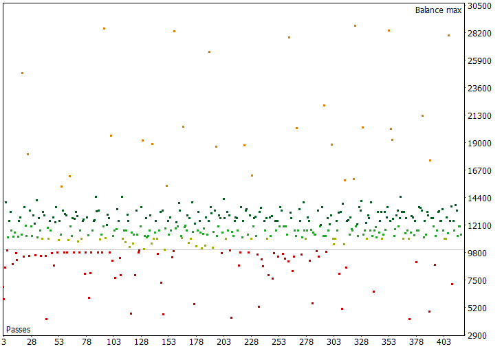
Backtest results graph
At a glance, we can see that there are many profitable data points. It signifies that our trading premise, parameter choices, and testing ranges have real credibility. The highest ending balance is 25356.81, with most data points clustering around the 12500 level for the one-year backtest at 1% risk per trade. The first 15 records, sorted by ending balance, are displayed below.
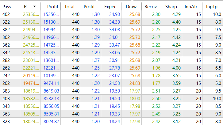
Optimization results
The records have about 440 trades, which is significant enough for intraday strategy analysis. The best-performing ATR percentages are 15 and 20, with 20 offering lower drawdowns. The worst-performing ATR percentage is 5 due to trading costs. ATR percentages of 30 to 50 are also generally profitable at higher take-profit multiples. Records without a take-profit, relying solely on the session close, are all unprofitable. Out of the 420 strategy parameter combinations, 344 (81.9%) are profitable. The graph of the best-performing strategy parameter combination along with backtest details is shown below.
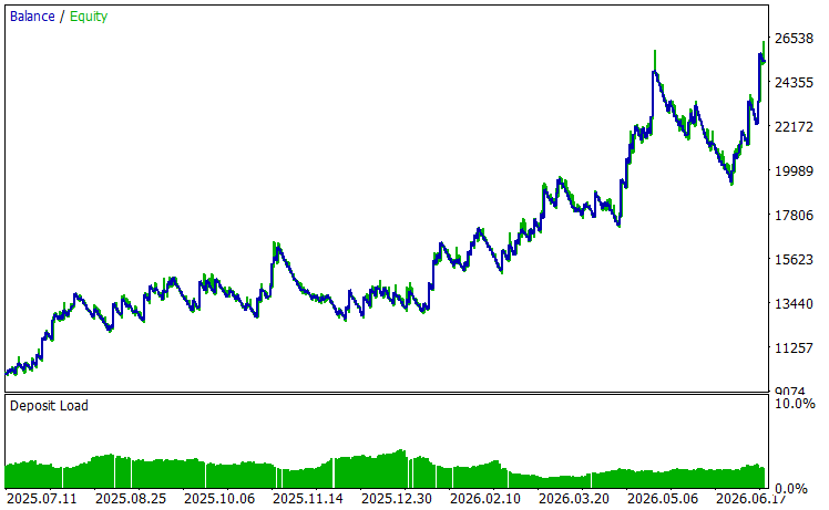
Best-performing strategy parameter combination
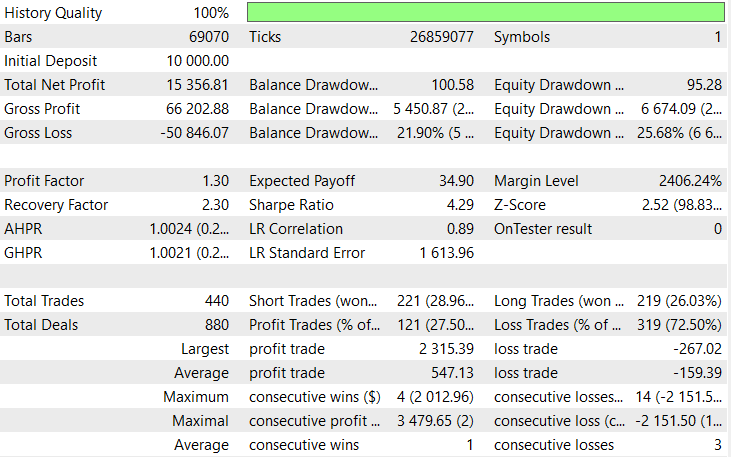
Best-performing backtest
The backtest has a net profit of 153.57% with a max equity drawdown of 25.68%. The dip towards the end of the graph may appear to be large, but this is a feature of the percent-based risk management. The strategy scales to higher position sizes with the accumulation of profits, and that is why the trough appears deeper than the previous troughs. The deposit load remains steady below 10% at 1:100 leverage, signifying that despite the increase in lot sizes, the relative margin deployment does not drastically increase. The overall win rate is 27.5%, which is expected as breakout trades are implicitly trend following. Short trades have a slightly higher win rate of 28.96% compared to the long trades' win rate of 26.03%.
Selecting parameters from backtest results depends on both quantitative metrics and trader constraints. Parameters can be chosen based on performance metrics such as profit factor and Sharpe ratio or operational constraints such as max drawdown and win rate. It is tempting to opt for the best-performing strategy parameters; however, there are chances that these records are swayed by outliers. To analyze outliers, we can either manually review the backtest trade logs or, more simply, evaluate the smoothness of the optimization surface.
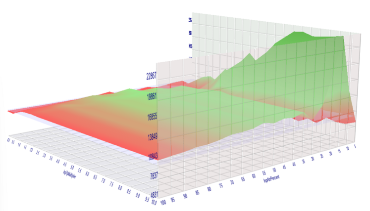
Optimization surface
The best-performing strategy parameters are 15 ATR percentage and 10 take-profit multiplier. We observe that the surface leading up to that point on the graph does not have sudden jumps. It can also be verified from the backtest records that take-profit multiples around 10 also have similar performances. So we can confirm that this is a good candidate for the optimal set.
The strategy prefers smaller ATR percentages, as evidenced by the backtest results. Smaller ATR multiples allow for larger relative price moves to be captured during breakouts while enabling higher position leverage. However, there is a limit to how small we can go. The results at 5% ATR were not profitable despite the advantages of a smaller ATR percentage, as the spread cost overwhelmed the trading gains. In general, intraday strategies are affected by costs, slippage, execution delay, and price gaps. The live strategy parameters could diverge from the ideal execution results that we have derived to test the premise. To analyze the sensitivity to costs, we run the best-performing parameter set with a 243 ms execution delay and simulated slippage.
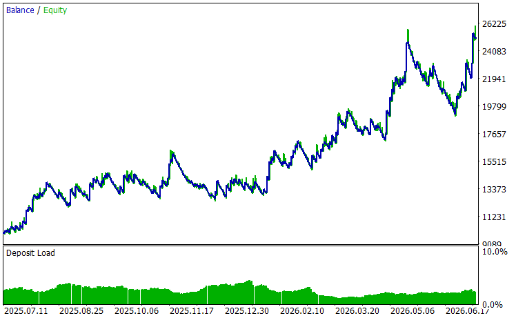
Graph of best-performing strategy parameters with simulated slippage
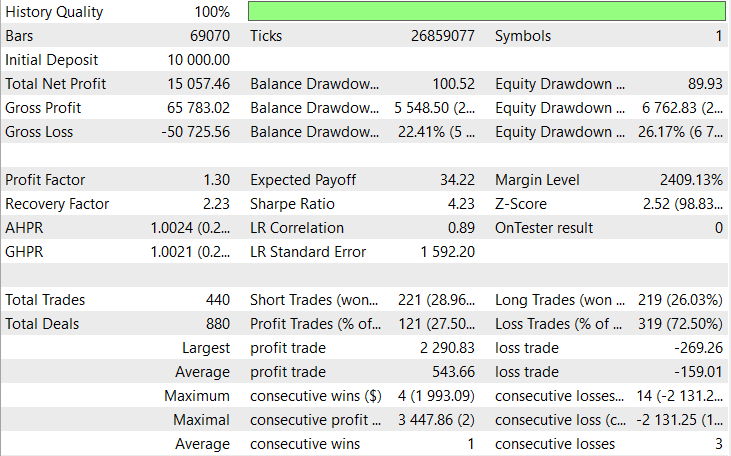
Backtest of the best-performing parameters with simulated slippage
The net profit percentage comes down by 3% to 150.57%, and the max equity drawdown increases by 0.49% to 26.17%. Our decision to cap at two trade attempts greatly helps in minimizing the effects of intraday cost consideration. Overall, from the test, we can say that the First Fractal Breakout strategy has the potential to generate returns even in non-ideal execution environments.
For a given ATR percentage, as the take-profit multipliers increase, the take-profit level becomes harder to reach, and the strategy increasingly relies on the fractal entries and session close for its edge. Notably, the top-performing strategy parameter combinations feature a high take-profit level. This indicates that the ideal behavior of the strategy is to derive its edge from a combination of the occasional high reward-risk wins and the daily close. The EA accumulates and categorizes the statistics of its trades based on closing reason. The breakdown of our best-performing parameter set as per the count of the closing reason is as follows.
| Long | Short | Total | |
|---|---|---|---|
| Stop-loss | 156 | 154 | 310 |
| Take-profit | 4 | 6 | 10 |
| Close Profit | 53 | 58 | 111 |
| Close Loss | 6 | 3 | 9 |
| Total | 219 | 221 | 440 |
Similarly, a breakdown of the gross profit and loss by the closing reason.
| Long | Short | Total | |
|---|---|---|---|
| Stop-loss | -25281.0 | -24902.67 | -50183.67 |
| Take-profit | 7642.26 | 8481.99 | 16124.25 |
| Close Profit | 24287.64 | 25790.99 | 50078.63 |
| Close Loss | -480.47 | -181.93 | -662.40 |
| Total | 6168.4 | 9188.4 | 15356.81 |
Out of the 121 profitable trades, 10 trades closed on the take-profit at a multiplier of 10. The remaining bulk of the profits came from the 111 profitable closes after the fractal entries. While the close profits constituted the most gross profits, the 10 profitable trades contributed 32.2% of the gross close profits. This reflects the dynamics of trend following, where a small fraction of wins seems to contribute a significant amount to the overall gains. An interesting observation is that only 9 of the 319 losing trades were at the session close. The closing losses contributed only 1.32% of the gross losses as the stop-loss hits. This suggests that first fractal entries combined with a small ATR percentage that avoid getting stopped out are likely to end the trading session in profit.
The correlation scatter plot of the Profit vs. Maximum Favorable Excursion (MFE) and Maximum Adverse Excursion (MAE) is shown below.
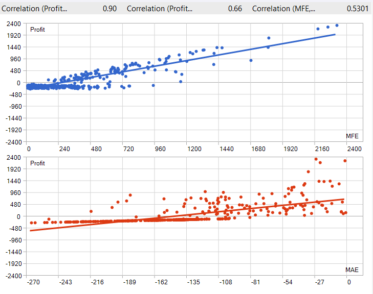
Correlation graph of Profit vs. MFE/MAE
The Profit vs. MFE scatter correlation of 0.90 indicates that the strategy converts favorable excursions into realized profit efficiently. The scatter is almost a straight line from the origin, staying tight all the way out to the largest trades. Eyeballing the fitted line, we can say that when a trade moves in its favor, the strategy captures 75% to 80% of the MFE rather than watching it round-trip. The giveback is modest, and this is a genuine point in favor of the high-reward-risk-plus-session-close exit strategy.
The weak Profit vs. MAE scatter correlation of 0.66 shows the signature expected from a cleanly working hard stop-loss. Once adverse excursion reaches the stop distance, the position is closed, and further downside stops mattering. The MAE chart near zero shows that the best trades have minimal adverse excursion. These trades are clean breakouts and are exited near their peak. These are precisely the trades we set out to catch with the First Fractal Breakout strategy.
Our findings so far indicate that the premise of fractals serving as the market's own record of its microstructure has encouraging quantitative evidence. However, what proportion of the results can be attributed to the intrinsic predictive nature of fractals, as opposed to the DAX simply performing well under general breakout methodologies? To isolate the structural value of fractals, we benchmark the system against the 15-minute ORB strategy.
The range limits for the ORB strategy are set from the high and low of the first 15 minutes of the session (9:00 to 9:15 for the DAX); all other parameters, trading attempt limits, risk management, and environment variables are kept the same as we did for the First Fractal Breakout.
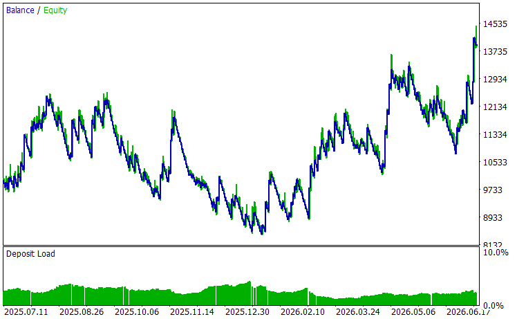
Graph of the 15-minute ORB strategy
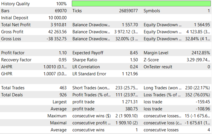
Backtest of the 15-minute ORB strategy
The 15-minute ORB strategy is profitable under similar conditions. The net profit is 39.12% at a max equity drawdown of 32.84%. By comparison, the fractal entry's net profit of 153.57% at a max equity drawdown of 25.68% fares significantly better. The 15-minute ORB relies solely on a fixed, time-based window; it frequently establishes arbitrary range limits regardless of the market structure. In contrast, the fractal approach adapts dynamically to the live local structure pivots. The comparative analysis empirically suggests that the First Fractal Breakout strategy is not merely an artifact of favorable index tailwinds.
Throughout this article we have developed, backtested, and rigorously analyzed the strategy using the DAX index. While our results are encouraging, the analysis thus far remains localized to in-sample data and a single asset class. This leaves us with two questions:
- How effective is the strategy across a completely different asset class?
- How do the optimized strategy parameters perform across unseen data?
To evaluate robustness and out-of-sample parameter validity, we run a 1:1 in-sample/out-of-sample test on Gold (XAUUSD). The duration is split into two equal halves for the backtest and forward test, respectively. As Gold exhibits strong directional trends in both the London and New York sessions, the start time is set at the London open and the end time is set 15 minutes prior to the New York close to avoid overnight funding costs. This large trading window is sufficient to capture the global intraday trends. The first 15 records of the backtest results are shown below. The optimal parameters, ATR percent 25 and take-profit multiplier 6 were chosen after analysis of outliers and performance metrics. This optimum set is tested for its parameter stability in the forward test. The complete details are provided in the table below.
| Parameter | Value |
|---|---|
| Symbol | XAUUSD |
| Timeframe | M5 |
| Backtest Period | 2025-07-10 to 2026-01-10 |
| Forward Period | 2026-01-10 to 2026-07-10 |
| Currency | USD |
| Initial Deposit | 10,000 |
| Leverage | 1:100 |
| Modeling | Every tick based on real ticks |
| Start Hour | 10 |
| Start Min | 0 |
| End Hour | 23 |
| End Min | 45 |
| Risk Percent Per Trade | 1 |
| ATR Period | 14 |
| ATR Percentage | 25 |
| TP Multiplier | 6.0 |
| Magic Number | 12345 |
The test results are shown below.
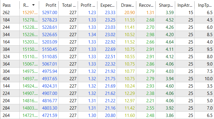
First 15 records of the backtest sorted by ending balance
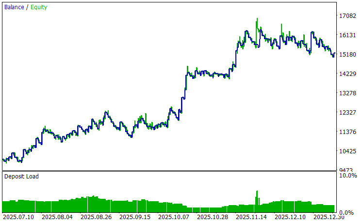
Backtest graph of the optimum parameters
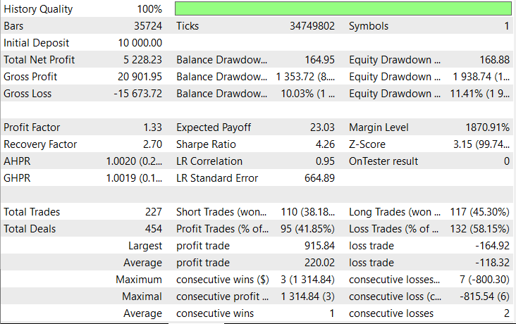
Backtest of the optimum parameters
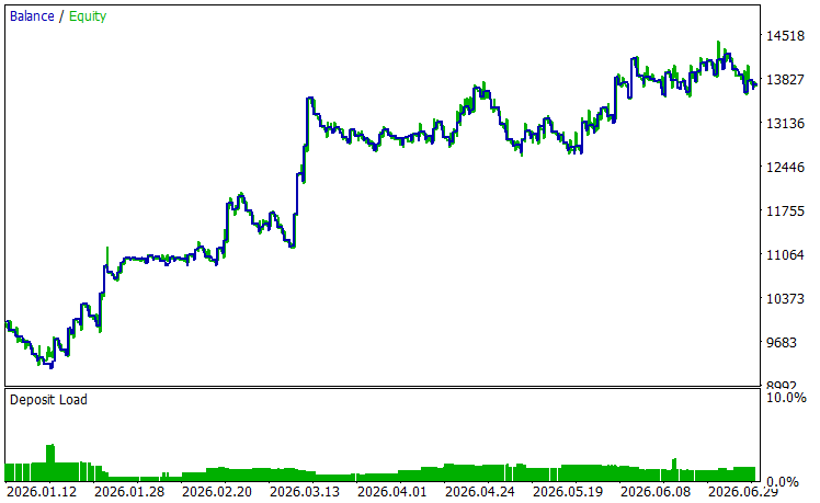
Forward test graph
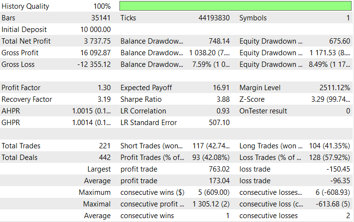
Forward test
The backtest and forward tests have 227 and 221 trades, respectively, which is sufficient for drawing conclusions regarding strategy performance. The backtest has a net profit of 52.28% at a max equity drawdown of 11.41% over the 6-month period. Compared to the DAX, the overall win rate is higher, 41.85% due to the lower take-profit multiplier. On the other hand, the forward test is also profitable with a net profit of 37.38% at a max equity drawdown of 8.49%.
To analyze parameter stability, we compare the performance metrics. The trade frequency across the two tests remains remarkably stable (227 vs. 221 trades). The core indicators of strategy health—namely profit factor (1.33 vs. 1.30) and win rate (41.85% vs. 42.08%) show virtually zero degradation when evaluated on out-of-sample data. While the forward test has lower returns, the recovery factor (2.70 vs. 3.19) has actually improved owing to the lower max equity drawdown (11.41% vs. 8.49%).
The forward test on XAUUSD offers compelling support for the First Fractal Breakout strategy, addressing concerns regarding single-asset overfitting and parameter stability. The comparable performance metrics on out-of-sample data suggest that the framework possesses the structural stability required to perform across unseen environments. While no tests can fully account for market regimes and execution frictions, our observations across all testing phases suggest that anchoring entries to market-structure fractals offers a viable mechanism for capturing intraday breakout momentum.
Conclusion
This article presented the comprehensive development, implementation, and systematic evaluation of the First Fractal Breakout trading strategy—an intraday approach that uniquely leverages Bill Williams market fractals to define breakout levels in a market-driven, adaptive manner. Through rigorous backtesting using 100% quality tick data over a one-year period, we provided preliminary evidence that fractal-drawn levels capture meaningful market breakout points and demonstrated the strategy's potential as a practical framework for systematic intraday trading.
The strategy can be extended by adding trailing stops, filters for range size, trading day and news events, variable stops based on trade direction, and multi-symbol and multi-timeframe analysis. In summary, the First Fractal Breakout strategy represents a theoretically sound and empirically validated approach to intraday breakout trading. The strategy is ripe for further live testing and walk-forward analysis and has the potential to become a reliable and sustainable component of a diversified algorithmic trading portfolio.
Warning: All rights to these materials are reserved by MetaQuotes Ltd. Copying or reprinting of these materials in whole or in part is prohibited.
This article was written by a user of the site and reflects their personal views. MetaQuotes Ltd is not responsible for the accuracy of the information presented, nor for any consequences resulting from the use of the solutions, strategies or recommendations described.

 Zero-Copy Tick Streaming (Part 1): Bridging MetaTrader 5 to Shared Memory with the Arrow C Data Interface
 Market Simulation: Position View (XI)
 Self-Optimizing Expert Advisors in MQL5 (Part 19): Parameter Optimization For Time-Lagged Independent Components Analysis (2)
 From Basic to Intermediate: Queues, Lists, and Trees (III)

- Free trading apps
- Over 8,000 signals for copying
- Economic news for exploring financial markets
You agree to website policy and terms of use