

Self-Optimizing Expert Advisors in MQL5 (Part 19): Parameter Optimization For Time-Lagged Independent Components Analysis (2)
 733
733
 0
0

This article addresses a practical engineering problem: how to suppress statistical noise in lagged market features and turn the resulting structure into a reproducible, deployable risk-aware trading application for MQL5. Our starting point is a simple pipeline that computes moving‑average (MA) lagged features, learns an ICA embedding, and feeds that embedding into a linear classifier. In practice, we observed two failure modes:
- The ICA parameters and the manifold-based clusters did not reliably improve out-of-sample trading performance
- Direct deployment of spectral clustering in MQL5 is challenging because the current skl2onnx converter does not support scikit-learn clustering objects.
To address these issues we set three explicit objectives:
- Select ICA parameters that maximize predictive performance under time‑series cross‑validation.
- Discover actionable market regimes directly in lagged MA data using spectral clustering and then learn a deployable surrogate for those regimes.
- Deliver reproducible ONNX artifacts and MQL5 integration so the regimes can drive dynamic position sizing and stop logic.
Key methodological choices include time‑series CV, a line search on cluster counts, a surrogate multi‑output classifier to bypass ONNX limitations, and careful validation to avoid reward‑hacking on sparse, imbalanced multi‑output labels.
Getting Started in MQL5
Our exploration starts by first writing an MQL5 script to fetch the historical market data we need. This script will be familiar to returning readers, as it is the same script we used in our first discussion. We have attached the script here to accommodate any readers that may be with us for the first time. The script fetches historical lagged market data and its smoothed moving-average indicator values. We will mostly rely on the indicator values.
//+------------------------------------------------------------------+
//|                                                    ICA Filtering |
//|                                      Copyright 2026, CompanyName |
//|                                       http://www.companyname.net |
//+------------------------------------------------------------------+
#property copyright "Copyright 2026, MetaQuotes Ltd."
#property link      "https://www.mql5.com"
#property version   "1.00"
#property script_show_inputs

//+------------------------------------------------------------------+
//| Inputs                                                           |
//+------------------------------------------------------------------+
input group "File Properties"
input(name="Number of Bars") int size = 10;

input group "Technical Indicators"
input(name="MA Period") int MA_PERIOD = 5;
input(name="MA Type") ENUM_MA_METHOD MA_TYPE = MODE_EMA;

//--- File name
string file_name = Symbol() + " Noise Filter.csv";

//--- Technical indicators
int      ma_h,ma_l,ma_o,ma_c,file_handle;
double   ma_h_reading[],ma_l_reading[],ma_o_reading[],ma_c_reading[];

//+------------------------------------------------------------------+
//| Our script execution                                             |
//+------------------------------------------------------------------+
void OnStart()
  {

//--- Initialize inidcators
   ma_h = iMA(Symbol(),PERIOD_CURRENT,MA_PERIOD,0,MA_TYPE,PRICE_HIGH);
   ma_l = iMA(Symbol(),PERIOD_CURRENT,MA_PERIOD,0,MA_TYPE,PRICE_LOW);
   ma_o = iMA(Symbol(),PERIOD_CURRENT,MA_PERIOD,0,MA_TYPE,PRICE_OPEN);
   ma_c = iMA(Symbol(),PERIOD_CURRENT,MA_PERIOD,0,MA_TYPE,PRICE_CLOSE);

   if(ma_h == INVALID_HANDLE || ma_l == INVALID_HANDLE ||ma_o == INVALID_HANDLE ||ma_c == INVALID_HANDLE)
     {
      //--- We failed to load the indicators
      Comment("Failed To Load Technical Indicators: ",GetLastError());
      return;
     }

   else
     {
      //---Write to file
      file_handle=FileOpen(file_name,FILE_WRITE|FILE_ANSI|FILE_CSV,",");

      for(int i=size;i>=1;i--)
        {

         //--- Update indicator values

         //--- High MA
         if(CopyBuffer(ma_h,0,i,6,ma_h_reading) <= 0)
           {
            Print("An error occurred when copying the High moving average buffer: ",GetLastError());
            return;
           }
         ArraySetAsSeries(ma_h_reading,true);

         //--- Open MA
         if(CopyBuffer(ma_o,0,i,6,ma_o_reading) <= 0)
           {
            Print("An error occurred when copying the Open moving average buffer: ",GetLastError());
            return;
           }
         ArraySetAsSeries(ma_o_reading,true);

         //--- Low MA
         if(CopyBuffer(ma_l,0,i,6,ma_l_reading) <= 0)
           {
            Print("An error occurred when copying the Low moving average buffer: ",GetLastError());
            return;
           }

         ArraySetAsSeries(ma_l_reading,true);

         //--- Close MA
         if(CopyBuffer(ma_c,0,i,6,ma_c_reading) <=0)
           {
            Print("An error occurred when copying the Close moving average buffer: ",GetLastError());
            return;
           }
         ArraySetAsSeries(ma_c_reading,true);

         //--- Fill in the column names
         if(i == size)
           {
            FileWrite(file_handle,
                      //--- Time
                      "Time",
                      //--- OHLC
                      "Open",
                      "High",
                      "Low",
                      "Close",
                      //--- OHLC Lag 1
                      "Open Lag 1",
                      "High Lag 1",
                      "Low Lag 1",
                      "Close Lag 1",
                      //--- OHLC Lag 2
                      "Open Lag 2",
                      "High Lag 2",
                      "Low Lag 2",
                      "Close Lag 2",
                      //--- OHLC Lag 3
                      "Open Lag 3",
                      "High Lag 3",
                      "Low Lag 3",
                      "Close Lag 3",
                      //--- OHLC Lag 4
                      "Open Lag 4",
                      "High Lag 4",
                      "Low Lag 4",
                      "Close Lag 4",
                      //--- OHLC Lag 5
                      "Open Lag 5",
                      "High Lag 5",
                      "Low Lag 5",
                      "Close Lag 5",
                      //--- Indicators
                      "MA O",
                      "MA H",
                      "MA L",
                      "MA C",
                      //--- Indicators lag 1
                      "MA O Lag 1",
                      "MA H Lag 1",
                      "MA L Lag 1",
                      "MA C Lag 1",
                      //--- Indicators lag 2
                      "MA O Lag 2",
                      "MA H Lag 2",
                      "MA L Lag 2",
                      "MA C Lag 2",
                      //--- Indicators lag 3
                      "MA O Lag 3",
                      "MA H Lag 3",
                      "MA L Lag 3",
                      "MA C Lag 3",
                      //--- Indicators lag 4
                      "MA O Lag 4",
                      "MA H Lag 4",
                      "MA L Lag 4",
                      "MA C Lag 4",
                      //--- Indicators lag 5
                      "MA O Lag 5",
                      "MA H Lag 5",
                      "MA L Lag 5",
                      "MA C Lag 5"
                     );
           }

         //--- Fill in the column values
         else
           {
            FileWrite(file_handle,
                      iTime(_Symbol,PERIOD_CURRENT,i),
                      //--- OHLC
                      iOpen(_Symbol,PERIOD_CURRENT,i),
                      iHigh(_Symbol,PERIOD_CURRENT,i),
                      iLow(_Symbol,PERIOD_CURRENT,i),
                      iClose(_Symbol,PERIOD_CURRENT,i),
                      //--- OHLC Lag 1
                      iOpen(_Symbol,PERIOD_CURRENT,i+1),
                      iHigh(_Symbol,PERIOD_CURRENT,i+1),
                      iLow(_Symbol,PERIOD_CURRENT,i+1),
                      iClose(_Symbol,PERIOD_CURRENT,i+1),
                      //--- OHLC Lag 2
                      iOpen(_Symbol,PERIOD_CURRENT,i+2),
                      iHigh(_Symbol,PERIOD_CURRENT,i+2),
                      iLow(_Symbol,PERIOD_CURRENT,i+2),
                      iClose(_Symbol,PERIOD_CURRENT,i+2),
                      //--- OHLC Lag 3
                      iOpen(_Symbol,PERIOD_CURRENT,i+3),
                      iHigh(_Symbol,PERIOD_CURRENT,i+3),
                      iLow(_Symbol,PERIOD_CURRENT,i+3),
                      iClose(_Symbol,PERIOD_CURRENT,i+3),
                      //--- OHLC Lag 4
                      iOpen(_Symbol,PERIOD_CURRENT,i+4),
                      iHigh(_Symbol,PERIOD_CURRENT,i+4),
                      iLow(_Symbol,PERIOD_CURRENT,i+4),
                      iClose(_Symbol,PERIOD_CURRENT,i+4),
                      //--- OHLC Lag 5
                      iOpen(_Symbol,PERIOD_CURRENT,i+5),
                      iHigh(_Symbol,PERIOD_CURRENT,i+5),
                      iLow(_Symbol,PERIOD_CURRENT,i+5),
                      iClose(_Symbol,PERIOD_CURRENT,i+5),
                      //--- Indicators
                      ma_o_reading[0],
                      ma_h_reading[0],
                      ma_l_reading[0],
                      ma_c_reading[0],
                      //--- Indicators lag 1
                      ma_o_reading[1],
                      ma_h_reading[1],
                      ma_l_reading[1],
                      ma_c_reading[1],
                      //--- Indicators lag 2
                      ma_o_reading[2],
                      ma_h_reading[2],
                      ma_l_reading[2],
                      ma_c_reading[2],
                      //--- Indicators lag 3
                      ma_o_reading[3],
                      ma_h_reading[3],
                      ma_l_reading[3],
                      ma_c_reading[3],
                      //--- Indicators lag 4
                      ma_o_reading[4],
                      ma_h_reading[4],
                      ma_l_reading[4],
                      ma_c_reading[4],
                      //--- Indicators lag 5
                      ma_o_reading[5],
                      ma_h_reading[5],
                      ma_l_reading[5],
                      ma_c_reading[5]
                     );
           }
        }
     }
//--- Close the file
   FileClose(file_handle);
  }
//+------------------------------------------------------------------+
Analyzing Our Historical Market Data
Let us get started with our analysis. First, we will import the standard Python libraries we need for statistical analysis.
#Load standard libraries
import pandas as pd
import numpy as np
import matplotlib.pyplot as plt
import seaborn as sns
Read in the historical market data we have on file.
#Read in the market data
data = pd.read_csv("/ENTER/YOUR/PATH/HERE/EURUSD Noise Filter.csv")
data
Group our market inputs. We will work exclusively with the moving average group, because in our first discussion this group of inputs appeared to be the easiest to model and the most informative.
#Group the inputs
OHLC = data.iloc[:,1:25].columns
MA   = data.iloc[:,25:49].columns
ALL  = data.iloc[:,1:].columns
Label the market data.
#Define our forecast horizon
HORIZON = 5

#Label the data with a real valued target
data['New Target'] = data['MA C'].shift(-HORIZON) - data['MA C']

#Label the data with a binary target
data['New Bin Target'] = 0
data.loc[data['New Target'] > 0,'New Bin Target'] = 1
Filter missing rows from our data matrix.
#Filter missing rows
data = data.iloc[:-HORIZON,:]
We split the data into training and test sets. The test set contains the last three years of data and is not used further in this discussion. We focus on trading performance on this held-out set rather than on statistical metrics. Therefore, we have no need to keep the test set.
#Train test split
train , _ = data.iloc[:-(365*3),:],data.iloc[-(365*3):,:]
Let us now load the statistical libraries we will need.
#Spectral clustering
from sklearn.cluster import SpectralClustering
#One hot encoding
from sklearn.preprocessing import OneHotEncoder as OHE
#Load statistical libraries
from sklearn.decomposition import FastICA as ICA
#Pipeline
from sklearn.pipeline import Pipeline
#Linear support vector classifier
from sklearn.svm import LinearSVC as LSVC
#Logistic regression (Linear Classifier)
from sklearn.linear_model import LogisticRegression as LR
#Linear discriminant analysis (Linear Classifier)
from sklearn.discriminant_analysis import LinearDiscriminantAnalysis as LDA
#Model selection utilities
from sklearn.model_selection import cross_val_score,TimeSeriesSplit,RandomizedSearchCV
Initialize the time series validation object.
#Initialize the time series split
tscv = TimeSeriesSplit(n_splits=5,gap=HORIZON)
We will now perform a line search evaluating our classification performance with a varying number of clusters. Spectral clustering is much more powerful than the KMeans algorithm we used in our first attempt. It can perform well even when clusters are nested and not well separated. The algorithm is sensitive to the weights and other parameters it was initialized with. Restarting the clustering routine with different parameters will yield different results.
#Max number of clusters we want to evaluate
EPOCHS = 10

#Keep track of our performance
clustering_score = []

#Evaluate our performance with different numbers of clusters
for i in np.arange(2,EPOCHS+1):
    #Define the clustering algorithm
    cls = SpectralClustering(n_clusters=i,random_state=0,assign_labels='cluster_qr')
    #Fit the clustering routine
    cls.fit(train.loc[:,MA])
    #Prepare the one hot encoder
    ohe = OHE(sparse_output=False)
    #Add the cluster labels
    train['Cluster'] = cls.labels_
    clustering_score.append(np.mean(cross_val_score(LR(),ohe.fit_transform(train[['Cluster']]),train['New Bin Target'],scoring='accuracy',cv=tscv)))
    print(clustering_score[i-2])
0.47965686274509806
0.4946078431372549
0.47524509803921566
Plotting our results shows a clear peak at 8 clusters. The red dashed line marks the performance level required for a 5% improvement over the initial accuracy we obtained by assuming only 2 clusters are optimal. It is possible to continue search over larger intervals of clusters, but this may be computationally expensive. Generally speaking, the algorithm runs slower and slower as the number of desired clusters increases.
plt.plot(clustering_score,color='black')
plt.axhline(clustering_score[0]*1.05,color='red',linestyle='--')
plt.ylabel('Cross-Validated accuracy out of 100%')
plt.xlabel('Number of Spectral Clusters')
plt.scatter(np.argmax(clustering_score),np.max(clustering_score),color='blue')
plt.title('Model Accuracy Against Spectral Clusters')
plt.grid()
Model Accuracy Against Spectral Cluster
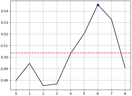
Figure 1: Our performance using spectral clusters to forecast smoothed market returns peaked at 8 clusters.
We will now assign cluster labels to our training set.
#Reproduce the best clustering setup
cls = SpectralClustering(n_clusters=8,assign_labels='cluster_qr')
ohe = OHE(sparse_output=False)
cls.fit(train.loc[:,MA])
train['Cluster'] = cls.labels_
Unfortunately, at the time of writing, the current version of the official ONNX converter for scikit-learn models, version 1.20.0, does not extend support to the library's clustering algorithms. To make use of the clustering information we have, we will train a surrogate supervised model to learn which cluster we are in, given market data. A link to the official documentation on all supported scikit-learn models is provided here.
To build a surrogate clustering model, we will first one-hot encode the cluster labels assigned to the training set. One-hot encoding the cluster labels creates a new matrix that has 8 columns, one for each cluster, and the same number of rows as the training set. Only the assigned cluster column will have a value of 1; all other columns will be set to 0. Let us assess our performance on each cluster.
#Create a dataframe to store our one hot encoded cluster labels
clusters = pd.DataFrame(ohe.fit_transform(train[['Cluster']]),columns=['Cluster 1','Cluster 2','Cluster 3','Cluster 4','Cluster 5','Cluster 6','Cluster 7','Cluster 8'])

#Performance classifying each cluster
performance = []

#Iterate over all clusters
for i in np.arange(8):
    c = 'Cluster '+str(i+1)
    performance.append(np.mean(cross_val_score(LDA(),train.loc[:,MA],clusters[c],scoring='accuracy',cv=tscv)))
Our results show remarkable performance on the first 7 clusters. Particularly, we almost achieved 100% accuracy on cluster 1, while our performance on cluster 8 is relatively dismal. Overall, our performance across all 8 clusters is above the 50% threshold of chance. This gives us confidence that our surrogate model is performing well, or does it?
While this methodology is intuitively appealing and sounds like a reasonable way of assessing our model, it is actually a numerical trap. I'll use this moment to engage the reader to think about why this may be an ineffective way of assessing our model's performance. Advanced readers may already see the dangers we face by assessing the model's performance this way. This step was taken deliberately to highlight a potential pitfall practitioners may unintentionally walk into. Do you think that our poor performance on cluster 8 is the critical error I am alluding to? In your opinion, what could possibly be wrong with the results we have produced?
sns.barplot(performance,palette='muted')
plt.xlabel('Cross-Validated Accuracy Classfying Clusters')
plt.ylabel('Accuracy Over Each Spectral Cluster')
plt.title('Our Ability To Identify Each Cluster In The Data')
plt.axhline(0.5,color='red',linestyle='--')
Our Ability to Identify Each Cluster in The Data
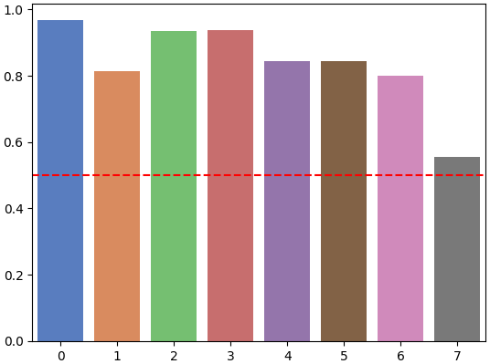
Figure 2: We seem to be classifying each spectral cluster well, but all is not as it seems.
I ask the reader to forgive me for teasing their imagination; I only did so as a writing technique to foster active learning for the reader. The critical error I am referring to is far more catastrophic than the low-performance levels we appear to have in cluster 8. To put it across concisely, the danger we face by assessing our performance on each cluster is that we are attempting to solve an imbalanced classification problem on a sparse, high-dimensional matrix.
If the issue is not yet clear, let us examine what went wrong and why this evaluation approach is discouraged. Understanding why this methodology is substandard will help you refrain from repeating it in your own private projects.
Let us closely recall the steps we have taken. Our spectral clustering algorithm identified 8 clusters of interest. We then built a data matrix with 8 columns, one for each cluster. The clusters we are working with are mutually exclusive. That means, for each row in the matrix of cluster labels, 7 columns will be set to 0 and only a single column will be assigned the value 1. This tells us that approximately 88% of all the values inside our cluster matrix are 0.
Therefore, if we consider each column individually, we will find that almost all its values are 0. This may allow a suboptimal model to produce astronomical performance levels by always predicting the label 0. This is a problem known as reward hacking, which we have discussed this extensively in our related series of articles "Overcoming The Limitation of Machine Learning (Part 1): Lack of Interoperable Metrics", a link to that article is provided, here.
So far, we have argued that this methodology is flawed. Now we provide evidence. Let us assess our performance on each cluster if we always predicted a vector of 0's. As we can see, a null classifier will produce an average performance level well above 80% if we assess our performance this way. In fact, the null classifier produced an accuracy of 97% on the first cluster.
#Accuracy metric
from sklearn.metrics import accuracy_score

#Let us observe how well we can perform by always predicting 0 on each cluster
null_performance = []
for i in np.arange(8):
    c = 'Cluster '+str(i+1)
    zeros = np.zeros(train.shape[0])
    null_performance.append(accuracy_score(zeros,clusters[c]))

sns.barplot(null_performance,palette='muted')
plt.xlabel('Spectral Cluster')
plt.ylabel('Accuracy of a null classifier')
plt.title('The accuracy of a Null Classifier on Each Cluster')
The Accuracy of a Null Classifier
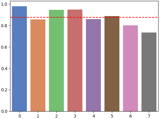
Figure 3: A model that has no understanding of the data and always predicts a vector of 0 outperformed us across all 8 clusters.
This makes it challenging to interpret how well you are performing on each cluster. Therefore, a better approach to follow is to instead measure your joint accuracy at classifying all 8 clusters at once. By doing so, our model will be making predictions on all 8 columns at once. Since one of these columns is guaranteed not to be zero, our performance metrics cannot be hacked by a model that forecasts a vector of 8 zeros across all samples.
This produced an accuracy of 84%. While this sounds like good performance, there is still one more check we need to make to ensure that the model is not hacking this reward by being biased and assigning most labels to the most common class. If any single spectral class accounts for more than 80% of all our observations, then we may be in trouble. Otherwise, if no single class has a contribution that is close to our accuracy level, then we can be confident our model is not hacking the cluster distribution to feign its skill.
from sklearn.neighbors import KNeighborsClassifier

multioutput_mean = np.mean(cross_val_score(KNeighborsClassifier(),train.loc[:,MA],clusters,cv=tscv,scoring='accuracy'))
multioutput_mean
0.8477941176470589
To calculate the portion of training samples that belong to each cluster, simply calculate the mean of the cluster matrix. The largest value in the vector of means represents the contribution of the largest cluster. The largest cluster, cluster 8, was assigned approximately 27% of the samples. That means the performance levels we obtained could not be recreated by always predicting the largest cluster. The model is demonstrating true skill.
largest_cluster = np.max(clusters.mean())
largest_cluster
0.2676056338028169
Keep track of the expected returns and risk levels associated with each cluster.
cls_return = []
cls_risk   = []
for i in np.arange(8):
    cls_return.append(train.loc[train['Cluster']==i,'C Target'].mean())
    cls_risk.append(train.loc[train['Cluster']==i,'C Target'].std())
It appears that clusters 1, 3 and 4 are associated with above-average returns. This information may be exploited to open larger positions when the intended trade and the expected cluster are aligned.
sns.barplot(cls_return,palette='muted')
plt.title('Average Return Per Spectral Cluster')
plt.xlabel('Spectral Cluster')
plt.ylabel('Expected 5-Day Return')
plt.axhline(np.mean(np.abs(cls_return)),color='red',linestyle='--')
plt.axhline(-np.mean(np.abs(cls_return)),color='red',linestyle='--')
Average Return Per Spectral Cluster
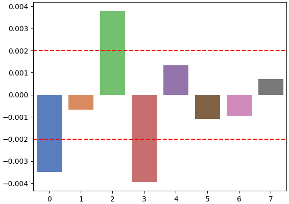
Figure 4: The expected return associated with each spectral cluster provides strong confirmation for our trades.
Not only that, but we can also learn which clusters are associated with risky market conditions. We can use this information to place trades with tighter stops when we are in clusters with above-average risk. These clusters may be closely associated with more volatile market conditions.
sns.barplot(cls_risk,palette='muted')
plt.axhline(np.mean(cls_risk),linestyle='--',color='red')
plt.ylabel('Expected Risk')
plt.xlabel('Spectral Cluster')
plt.title('Expected Risk Levels For Each Spectral Cluster')
Expected Risk Levels For Each Spectral Cluster
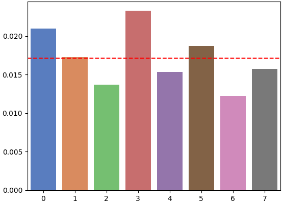
Figure 5: The risk levels associated with each cluster help us select tight stop-losses when market conditions are expected to be volatile.
Optimizing Our ICA Parameters
Let us now turn our attention to optimizing the parameters of the ICA algorithm. We will use a pipeline to efficiently search for parameter settings of the algorithm and then assess the improvements made on a linear classifier attempting to forecast smoothed market returns.pipe = Pipeline([
('ica',ICA(random_state=0)),
('lr',LR())
]) We will first define the parameters accepted by the ICA algorithm. These parameters change the low-dimensional representation the algorithm learns from the data and may allow us to learn non-linear relationships. With the parameter distribution defined, we set up a RandomizedSearchCV object to search the parameter space. The randomized search object allows us to efficiently choose between the quality of the results found and the time taken to compute by adjusting the number of iterations we permit. More iterations yield higher-quality results.
#Define the parameter distribution we want to search over
param_dist = {
    'ica__n_components':np.arange(1,len(MA)),
    'ica__tol':np.logspace(-10,2,10),
    'ica__algorithm':['parallel','deflation'],
    'ica__whiten':['arbitrary-variance','unit-variance'],
    'ica__fun':['logcosh','exp','cube'],
    'ica__whiten_solver':['svd','eigh']
}

#Configure the random search
rscv = RandomizedSearchCV(
    pipe,
    param_distributions=param_dist,
    n_iter=90,
    cv=tscv,
    scoring='accuracy',
    n_jobs=-1
)

#Perform the search for optimal ICA parameters
rscv_res = rscv.fit(train.loc[:,MA],train.loc[:,'New Bin Target'])
With the search complete, we store the best ICA settings we found and create a utility function that returns the optimal ICA configuration.
def get_optimal_ica():
    return(ICA(whiten_solver=rscv_res.best_params_['ica__whiten_solver'],
               whiten=rscv_res.best_params_['ica__whiten'],
               tol=rscv_res.best_params_['ica__tol'],
               n_components=rscv_res.best_params_['ica__n_components'],
               fun=rscv_res.best_params_['ica__fun'],
               algorithm=rscv_res.best_params_['ica__algorithm'],
              random_state=0))
Let us now encode our historical market data to its ICA manifold. Our performance was optimized at 9 components.
#Fetch our optimal ICA encoder
ica_enc = get_optimal_ica()

#Transform the data to its manifold
manifold = pd.DataFrame(ica_enc.fit_transform(train.loc[:,MA]),columns=['ICA 1','ICA 2','ICA 3','ICA 4','ICA 5','ICA 6','ICA 7','ICA 8','ICA 9'])
Tuning Our Models
We are now ready to start optimizing the statistical models we will need for our trading application. First, import the model we will use.from sklearn.neighbors import KNeighborsRegressor as KNR
Then initialize each model. Note that the surrogate clustering model was set to 10 neighbors because this is the same number of neighbors that were considered by the original spectral clustering algorithm.
#Initialize the model
#First model learns to cluster the data
clustering_model = KNR(n_jobs=-1,n_neighbors=10)
#Second model learns to project the ICA embeddings
ica_model = KNR(n_jobs=-1)
#Last model learns to forecast returns from approximate ICA embeddings
returns_model = KNR(n_jobs=-1)
Define the parameters to be searched over. We want to keep the number of neighbors on the clustering model fixed at 10.
#Initialize the parameters to be searched
clustering_param_distribution = {
'weights':['uniform','distance'],
'algorithm':['auto','ball_tree','kd_tree','brute'],
'leaf_size':[10,20,30,40,50,60,70,80]
}

param_distribution = {
'n_neighbors':[5,10,15,20,30,50,90,150],
'weights':['uniform','distance'],
'algorithm':['auto','ball_tree','kd_tree','brute'],
'leaf_size':[10,20,30,40,50,60,70,80]
}
We will now search and fit the best parameters found for each model
#Initialize the random search object
rscv = RandomizedSearchCV(clustering_model,clustering_param_distribution,random_state=0,n_iter=90,cv=tscv,n_jobs=-1,scoring='neg_mean_squared_error')

#Search
results = rscv.fit(train.loc[:,MA],clusters)

#Fit the model
clustering_model = KNR(weights=results.best_params_['weights'],leaf_size=results.best_params_['leaf_size'],algorithm=results.best_params_['algorithm'])
clustering_model.fit(train.loc[:,MA],clusters)

#Initialize the random search object
rscv = RandomizedSearchCV(ica_model,param_distribution,random_state=0,n_iter=90,cv=tscv,n_jobs=-1,scoring='neg_mean_squared_error')

#Search
results = rscv.fit(train.loc[:,MA],manifold)
ica_model = KNR(weights=results.best_params_['weights'],n_neighbors=results.best_params_['n_neighbors'],leaf_size=results.best_params_['leaf_size'],algorithm=results.best_params_['algorithm'])

#Fit the model
ica_model.fit(train.loc[:,MA],manifold)

#Store approximate ICA embeddings
ica_predictions = pd.DataFrame(ica_model.predict(train.loc[:,MA]))

#Initialize the random search object
rscv = RandomizedSearchCV(returns_model,param_distribution,random_state=0,n_iter=90,cv=tscv,n_jobs=-1,scoring='neg_mean_squared_error')

#Search
results = rscv.fit(ica_predictions,train.loc[:,'New Target'])

#Fit the model
returns_model = KNR(weights=results.best_params_['weights'],n_neighbors=results.best_params_['n_neighbors'],leaf_size=results.best_params_['leaf_size'],algorithm=results.best_params_['algorithm'])
returns_model.fit(ica_predictions,train.loc[:,'New Target'])
Exporting To ONNX
ONNX stands for Open Neural Network Exchange. It is a widely adopted industry standard for building and sharing machine models in a language-agnostic manner. Hopefully, in our future discussion the ONNX converter for scikit-learn will allow us to directly convert scikit-learn clustering algorithms into their ONNX representations. Install the necessary libraries if you have not already done so.
pip install onnx onnxruntime skl2onnx
Import the ONNX conversion libraries.
import onnx
from skl2onnx.common.data_types import FloatTensorType
from skl2onnx import convert_sklearn
Define the input and output shapes for our models.
clustering_initial_types = [('float_input',FloatTensorType([1,train.loc[:,MA].shape[1]]))]
clustering_final_types = [('float_output',FloatTensorType([1,clusters.shape[1]]))]

ica_initial_types = [('float_input',FloatTensorType([1,train.loc[:,MA].shape[1]]))]
ica_final_types = [('float_output',FloatTensorType([1,manifold.shape[1]]))]

returns_initial_types = [('float_input',FloatTensorType([1,manifold.shape[1]]))]
returns_final_types = [('float_output',FloatTensorType([1,1]))]
Save the ONNX files to disk. And we are now ready to assess the changes we have made on out-of-sample real market data.
onnx_proto = convert_sklearn(clustering_model,initial_types=clustering_initial_types,final_types=clustering_final_types,target_opset=12)
onnx.save(onnx_proto,'EURUSD SC KNR.onnx')

onnx_proto = convert_sklearn(ica_model,initial_types=ica_initial_types,final_types=ica_final_types,target_opset=12)
onnx.save(onnx_proto,'EURUSD ICA KNR.onnx')

onnx_proto = convert_sklearn(returns_model,initial_types=returns_initial_types,final_types=returns_final_types,target_opset=12)
onnx.save(onnx_proto,'EURUSD SR KNR.onnx')
Implementing Our Improvements in MQL5
We will now modify our trading application to take advantage of the new knowledge we have. Our application has over 500 lines of code. It would not be fair for returning readers that we review all 500 lines of code again. To avoid boring the returning audience, we will focus on the parts of our application that have changed significantly. At this point I will have to ask readers that are joining us for the first time to refer to our opening discussion if they desire to learn more about the code sections in the application that have been omitted from this discussion. A handy link to that discussion is provided here. The first change we will make will be to import the new ONNX model we have created.
//+------------------------------------------------------------------+
//| Resources                                                        |
//+------------------------------------------------------------------+
#resource "\\Files\\ICA Filtering\\EURUSD_ICA_KNR.onnx" as const uchar onnx_ica_proto[];
#resource "\\Files\\ICA Filtering\\EURUSD_SR_KNR.onnx" as const uchar onnx_returns_proto[];
#resource "\\Files\\ICA Filtering\\EURUSD_SC_KNR.onnx" as const uchar onnx_cluster_proto[];
Now we will also define important global variables that our application needs. Excluding the omitted code that has not changed, our global variables capture the new input shapes of our ONNX models and the statistical properties of our 8 spectral clusters.
//+------------------------------------------------------------------+
//| Global variables                                                 |
//+------------------------------------------------------------------+
//--- Fixed application variables
const int         ica_inputs = 24;
const int         ica_outputs = 9;
const int         returns_outputs = 1;
const int         cluster_outputs = 8;
const int         cluster_inputs = 24;

//--- Statistical market variables
double cluster_returns[] = {-0.003485849056603773,-0.0006836746143057491,0.003801236363636362,-0.003949062500000002,
                            0.0013250284900284896,-0.001098351254480287,-0.0009670449897750509,0.0007132494279176205
                           };
double cluster_risk[]    = {0.02095106970188371,0.017269570577721948,0.013691089299360098,0.023310184761761357,
                            0.015326219706248784,0.01875361535381102,0.01221513524812602,0.01572018673425591
                           };
double average_cluster_risk = 0.017154633922896106;
When our application is initialized for the first time, we will call this dedicated utility method that is responsible for setting up our ONNX models. Most of this code is familiar to our returning readers; the main change is that we have added a third model for predicting which cluster we are currently in. We set up our models from the ONNX buffers and define the input and output shapes according to the global variables we defined.
//+------------------------------------------------------------------+
//| Prepare our ONNX models for inferencing                          |
//+------------------------------------------------------------------+
bool LoadOnnxModels(void)
  {

//--- ONNX Models
   onnx_ica_model     = OnnxCreateFromBuffer(onnx_ica_proto,ONNX_DATA_TYPE_FLOAT);
   onnx_returns_model = OnnxCreateFromBuffer(onnx_returns_proto,ONNX_DATA_TYPE_FLOAT);
   onnx_cluster_model = OnnxCreateFromBuffer(onnx_cluster_proto,ONNX_DATA_TYPE_FLOAT);

//--- Validate the ONNX model handlers
   if(onnx_cluster_model == INVALID_HANDLE)
     {
      return(false);
     }

   if(onnx_returns_model == INVALID_HANDLE)
     {
      return(false);
     }

   if(onnx_ica_model == INVALID_HANDLE)
     {
      return(false);
     }

//--- Validate the ONNX model shapes
   ulong onnx_ica_input_shape[] = {1,ica_inputs};
   ulong onnx_ica_output_shape[] = {1,ica_outputs};
   ulong onnx_returns_output_shape[] = {1,returns_outputs};
   ulong onnx_cluster_input_shape[] = {1,cluster_inputs};
   ulong onnx_cluster_output_shape[] = {1,cluster_outputs};

   if(!OnnxSetInputShape(onnx_cluster_model,0,onnx_cluster_input_shape))
     {
      Print("Failed to set the correct ONNX Spectral Clustering model input shape: ",GetLastError());
      return(false);
     }

   if(!OnnxSetOutputShape(onnx_cluster_model,0,onnx_cluster_output_shape))
     {
      Print("Failed to set the correct ONNX Spectral Clustering model output shape: ",GetLastError());
      return(false);
     }

   if(!OnnxSetInputShape(onnx_ica_model,0,onnx_ica_input_shape))
     {
      Print("Failed to set the correct ONNX ICA model input shape: ",GetLastError());
      return(false);
     }

   if(!OnnxSetOutputShape(onnx_ica_model,0,onnx_ica_output_shape))
     {
      Print("Failed to set the correct ONNX ICA model output shape: ",GetLastError());
      return(false);
     }

   if(!OnnxSetInputShape(onnx_returns_model,0,onnx_ica_output_shape))
     {
      Print("Failed to set the correct ONNX smoothed returns model input shape: ",GetLastError());
      return(false);
     }

   if(!OnnxSetOutputShape(onnx_returns_model,0,onnx_returns_output_shape))
     {
      Print("Failed to set the correct ONNX smoothed returns model output shape: ",GetLastError());
      return(false);
     }

//--- Prepare ONNX model I/O
   onnx_ica_inputs = vectorf::Zeros(ica_inputs);
   onnx_ica_outputs = vectorf::Zeros(ica_outputs);
   onnx_return_outputs = vectorf::Zeros(returns_outputs);
   onnx_cluster_outputs = vectorf::Zeros(cluster_outputs);

//--- Everything went well
   return(true);
  }
If our application is no longer in use, we must release the technical indicators and the ONNX models that were allocated resources. In the code excerpt below, we only focused on the new ONNX models that have to be released.
//+------------------------------------------------------------------+
//| Free up all resources we are no longer using                     |
//+------------------------------------------------------------------+
bool ReleaseResources(void)
  {
   if(!OnnxRelease(onnx_cluster_model))
     {
      Print("An error occurred when releasing the ONNX Cluster model: ",GetLastError());
      return(false);
     }

   if(!OnnxRelease(onnx_ica_model))
     {
      Print("An error occurred when releasing the ONNX ICA model: ",GetLastError());
      return(false);
     }

   if(!OnnxRelease(onnx_returns_model))
     {
      Print("An error occurred when releasing the ONNX Smoothed Returns model: ",GetLastError());
      return(false);
     }
   return(true);
  }
When prices update, we detect the start of a new daily candle by comparing timestamps with the previous day. Then we fetch updated forecasts from all 3 of our statistical models.
//+------------------------------------------------------------------+
//| Expert tick function                                             |
//+------------------------------------------------------------------+
void OnTick()
  {
//--- Update our time reading
   time_stamp = iTime(Symbol(),PERIOD_D1,1);
   static datetime previous_time_stamp;

   if(previous_time_stamp != time_stamp)
     {
      //--- Update the time stamp
      previous_time_stamp = time_stamp;

      //--- Fetch updated indicator readings
      if(!UpdateMarketData())
        {
         Print("An error occurred while trying to update indicator readings: ",GetLastError());
         return;
        }

      //--- Prepare the inputs for our ONNX models
      if(!FetchModelData())
        {
         Print("An error occurred while trying to fetch our ONNX model data: ");
         return;
        }

      //--- Approximate our ICA embeddings
      if(!OnnxRun(onnx_ica_model,ONNX_DATA_TYPE_FLOAT,onnx_ica_inputs,onnx_ica_outputs))
        {
         Print("Failed to approximate ICA embedings: ",GetLastError());
         return;
        }

      //--- Identify the cluster we are in
      else
         if(!OnnxRun(onnx_cluster_model,ONNX_DATA_TYPE_FLOAT,onnx_ica_inputs,onnx_cluster_outputs))
           {
            Print("Failed to identify Spectral Cluster: ",GetLastError());
            return;
           }

         else
           {
            //--- Forecast smoothed market returns from approximate ICA embeddings
            if(!OnnxRun(onnx_returns_model,ONNX_DATA_TYPE_FLOAT,onnx_ica_outputs,onnx_return_outputs))
              {
               Print("Failed to forecast market returns: ",GetLastError());
               return;
              }

            else
              {
               SetupPosition();
              }
           }
     }
  }
//+------------------------------------------------------------------+
We also define 2 new utility functions responsible for opening our positions with a specified lot size and stop loss width.
//+------------------------------------------------------------------+
//| Enter short positions                                            |
//+------------------------------------------------------------------+
void Sell(double lot,double sl_width)
  {
   if(!Trade.Sell(lot,Symbol(),bid,ask+(sl_width*atr[0]),ask-(sl_width*atr[0])))
     {
      Print("Something went wrong while setting up our sell position: ",GetLastError());
      return;
     }
  }

//+------------------------------------------------------------------+
//| Enter long positions                                             |
//+------------------------------------------------------------------+
void Buy(double lot,double sl_width)
  {
   if(!Trade.Buy(lot,Symbol(),ask,bid-(sl_width*atr[0]),bid+(sl_width*atr[0])))
     {
      Print("Something went wrong while setting up our buy position: ",GetLastError());
      return;
     }
  }
Our trade-entry rules have changed. First, we identify the current cluster using the clustering model. Then we will retrieve the expected return and risk levels associated with the identified cluster. Next, we check the entry signal from the model that forecasts smoothed returns using the approximate ICA embeddings.
We use the largest lot size and widest stop-loss when the trade direction matches the cluster's expected return and the cluster risk is below average. Otherwise, if expected cluster return aligns with our desired trade, but the cluster risk is above average, we will reduce our lot size and employ a tighter stop-loss. Finally, under the worst-case entry condition, we will then use the smallest lot size and stop-loss width to preserve our trading capital.
//+------------------------------------------------------------------+
//| Execute our trade order                                          |
//+------------------------------------------------------------------+
void EnterTrade(void)
  {
//--- Let's keep track of the cluster expectations
   int         current_cluster    = (int) onnx_cluster_outputs.ArgMax();
   double expected_cluster_return = cluster_returns[current_cluster];
   double expected_cluster_risk   = cluster_risk[current_cluster];

//--- Long entries
   if(onnx_return_outputs[0] > 0)
     {
      //--- Best entry conditions possible
      if((expected_cluster_return > 0) && (expected_cluster_risk < average_cluster_risk))
        {
         Buy(0.03,2);
         return;
        }

      //--- Risky entry conditions, reduce the lot size and stop loss width
      else
         if((expected_cluster_return > 0) && (expected_cluster_risk > average_cluster_risk))
           {
            Buy(0.02,1.5);
            return;
           }

         //--- Worst possible entry conditions, use the smallest lot size and stop loss width
         else
           {
            Buy(0.01,1);
            return;
           }
     }

//--- Short entries
   if(onnx_return_outputs[0] < 0)
     {
      //--- Best entry conditions possible
      if((expected_cluster_return < 0) && (expected_cluster_risk < average_cluster_risk))
        {
         Sell(0.03,2);
         return;
        }
      //--- Risky entry conditions, reduce the lot size and stop loss width
      else
         if((expected_cluster_return < 0) && (expected_cluster_risk > average_cluster_risk))
           {
            Sell(0.02,1.5);
            return;
           }
         //--- Worst possible entry conditions, use the smallest lot size and stop loss width
         else
           {
            Sell(0.01,1);
            return;
           }
     }
  }
Backtesting Our Application
Let us now test our trading strategy. We will load the last 3 years of market data available. The reader should recall that this corresponds to the test set that we dropped when we constructed our models. Additionally, this also aligns with the same test period we selected for our previous discussion. 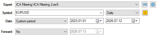
Figure 6: The backtest dates we will use to assess our application.
We will test our application with realistic settings to emulate live trading. To achieve this end, we will set our delay setting to random delay and model every tick based on real ticks. This gives the closest emulation of real market conditions possible.
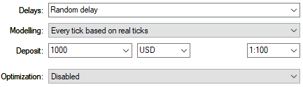
Figure 7: The test conditions we will use are selected to emulate real market conditions.
The equity curve produced by our trading strategy is depicted in the figure below. The strategy has a clear positive growth trend over the duration of the backtest. Although it did face challenging periods of drawdown, the application did not apply excessive strain on the account equity even though it had complete control over the lot size and stop-loss width. Additionally, the application recovered from all drawdown periods it encountered.
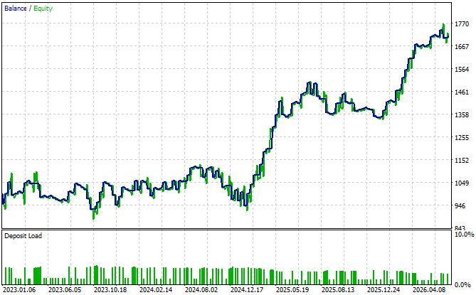
Figure 8: The equity curve produced by our trading strategy.
The detailed performance statistics show several improvements. For example, our initial version of the strategy produced a Sharpe Ratio of 0.62, while this revised version of our application produced a Sharpe Ratio of 0.8. This means that our application was changing its risk parameters efficiently. Additionally, the total number of trades increased from 69 to 128 trades over the same backtest period; this implies that we are uncovering more signal in the same amount of time. Lastly, and most importantly, our average and largest losing trades were meaningfully smaller than their counterparts. This demonstrates the potential held by unsupervised learning algorithms to direct our strategies.
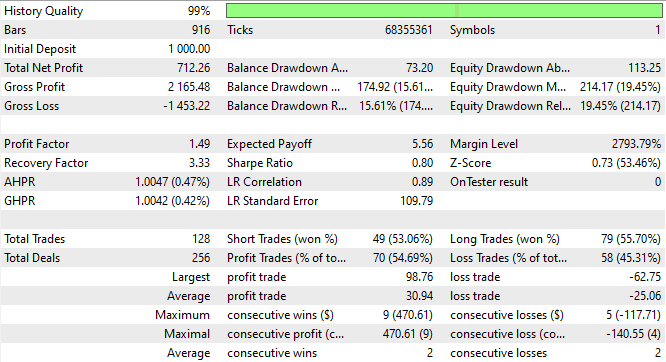
Figure 9: A detailed statistical table of our performance over the out-of-sample backtest window.
Conclusion
We provided an end-to-end, reproducible workflow for turning unsupervised structure in lagged MA features into deployable, risk-aware trading logic. Concretely, the reader obtains:
- A procedure to choose the number of spectral clusters by time‑series cross‑validation.
- Diagnostics and a practical avoidance strategy for the imbalanced multi‑output trap (do not evaluate one sparse column at a time; use joint multi‑output accuracy and check class priors).
- An interpretable way to optimize ICA hyperparameters via RandomizedSearchCV inside a pipeline that uses classifier performance as the objective.
- Three ONNX models (surrogate cluster predictor, ICA approximator, smoothed‑return regressor) to load in MQL5 for analyzing market regimes.
- A concrete MQL5 integration that uses cluster expected return and risk to adjust lot size and stop width. In backtests the revised system increased Sharpe ratio, raised trade frequency, and reduced important loss statistics, indicating better use of regime information.
There are a few caveats the reader should be aware of after reading this article. Foremost, our trading strategy implicitly assumes that the spectral cluster statistics obtained remain close to stationary over time, this may require validation over a longer test period. Additionally, the spectral clustering algorithm we employed is known to be sensitive to its initial conditions. Therefore, restarting the clustering procedure with different settings may render improved performance. These recommendations should be worthwhile for practitioners that have sufficient computational resources. If support for clustering objects is eventually included in the skl2onnx library, then our surrogate approach may need to be revised. All in all, this article's artifacts should be completely reproducible by the reader.
| File Name | File Description |
|---|---|
| EURUSD_SC_KNR.onnx | The ONNX model we created to identify which spectral cluster we are in. |
| EURUSD_ICA_KNR.onnx | This was the ONNX model responsible for approximating the current ICA embeddings. |
| EURUSD_SR_KNR.onnx | Our last ONNX model which forecasted smoothed market returns given approximate ICA embeddings. |
| ICA Filtering 2.mq5 | The trading application we designed to implement our unsupervised trading strategy. |
| statistical-noise-filter-2-optimization.ipynb | The Jupyter Notebook we used to analyze our historical market data and export our ONNX models. |
| ICA Filtering.mq5 | The MQL5 script we wrote to fetch the historical market data we needed for our analysis. |
Warning: All rights to these materials are reserved by MetaQuotes Ltd. Copying or reprinting of these materials in whole or in part is prohibited.
This article was written by a user of the site and reflects their personal views. MetaQuotes Ltd is not responsible for the accuracy of the information presented, nor for any consequences resulting from the use of the solutions, strategies or recommendations described.

 Machine Learning Under Constraint (Part 2): Calibrating Position Size to the Remaining Drawdown Budget
 Zero-Copy Tick Streaming (Part 1): Bridging MetaTrader 5 to Shared Memory with the Arrow C Data Interface
 Tables in the MVC Paradigm in MQL5: Symbol Correlation Table
 First Fractal Breakout — Intraday Strategy, Expert Advisor and Backtesting

- Free trading apps
- Over 8,000 signals for copying
- Economic news for exploring financial markets
You agree to website policy and terms of use