Markov Chain-Based Matrix Forecasting Model

Over the past decade, we have seen the triumph of neural networks and deep learning. But what if I told you that there is an even deeper level of market analysis? This is a level where advanced mathematical constructs meet classical Markov theory, and ancient Fibonacci harmonies are woven into self-learning genetic algorithms.

Financial markets are a kaleidoscope of chaos and order, intertwined in a single dance. Classical statistical approaches often founder on the reefs of market unpredictability, and neural networks, for all their sophistication, too often remain mysterious "black boxes". Between these extremes, there is a middle ground: probabilistic models built on the idea that markets retain information about their past through their current state. It is one of these models — a matrix iterative forecasting model based on Markov chains — that will be discussed in this study.

Our model combines the elegance of mathematical probability theory with the practicality of machine learning, representing the market as a system of transitions between discrete states. It is inspired by the fundamental observation that the market, despite its apparent randomness, contains hidden patterns that manifest themselves in various combinations of technical indicators, time cycles, and volume.

Mathematical foundations: From Markov to Wall Street

Andrey Markov, a prominent mathematician of the early 20th century, while working on probability theory, developed a concept that, a century later, became one of the cornerstones of modern financial mathematics. In developing the theory of stochastic processes, he studied sequences of events where the future depends only on the current state of the system, but not on previous history. This fundamental property — the absence of "memory" of the past beyond the current state — was called the "Markov property" and formed the basis of a whole class of models.

A Markov chain is a mathematical system that transitions from one state to another depending on probabilistic rules. If we imagine the possible states of a system as points in space, then the Markov chain describes the probabilities of movement between them. The stunning elegance of this concept lies in its ability to model incredibly complex processes through simple probabilistic mechanics.

Mathematically, a Markov chain is defined through a matrix of transition probabilities P, where the element P(i,j) represents the probability of transition from state i to state j. The key equation of a Markov chain can be written as:

π(t+1) = π(t) · P

where π(t) is the vector of probabilities of the system being in each of the states at time t.

From discrete states to continuous processes

Classical Markov chains operate with discrete states and discrete time, making them ideal for modeling systems such as price levels, market regimes, or trading sessions. However, the theory of Markov processes is not limited to discrete models. There are continuous Markov processes, the most famous of which is the Wiener process, a mathematical model of Brownian motion that underlies the famous Black-Scholes model for option pricing.

Hidden Markov Models (HMMs) represent another important extension, where the true state of the system is not directly observable, but only only indirect observations are available. This is particularly relevant for financial markets, where true market "regimes" (e.g. "bullish trend" or "consolidation") are not directly observable, but can only be inferred from observed price movements and volumes.

Financial markets provide an ideal testing ground for the application of Markov models. The efficient market hypothesis in its weak form states that future prices cannot be predicted from past prices, which effectively postulates the Markov property for price series. Although the full conformity of markets to a Markov process remains a matter of debate, empirical evidence confirms that for many practical problems, Markov approximations produce surprisingly accurate results.

In the context of trading, Markov models have found application in various aspects:

• Price movement forecasting - using historical statistics of market transitions to predict likely future movements.
• Market regime detection – automatic classification of the current market state as trending, sideways or transitional.
• Trading system optimization - adjusting strategy parameters depending on the identified market state.
• Risk assessment - calculation of the probabilities of large price movements based on the current state and known transition statistics.

Transition matrix: Algebra of market probabilities

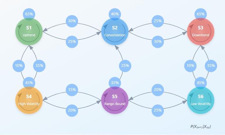
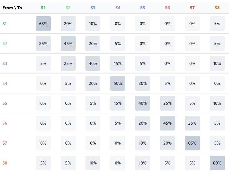
The central element of a Markov model is the transition matrix — a table in which the rows correspond to current states, the columns to future states, and the elements represent the probabilities of the corresponding transitions. For a financial market divided into n states, the transition matrix P has size n×n, where each row sums to one (since the system should transition to some state).

The strength of the Markov approach lies in the ability to apply this matrix iteratively to obtain multi-step forecasts. The probability of transition from state i to state j after k steps can be calculated as the corresponding element of the P^k matrix (P to the power k). This allows us to look further into the future, although the accuracy of predictions usually decreases as the forecast horizon increases.

Of particular interest is the limit behavior of the Markov chain as k→∞, which describes the long-term equilibrium distribution of state probabilities. For ergodic chains (where from any state one can reach any other in a finite number of steps) there exists a unique stationary distribution π* satisfying the equation:

π* = π* · P

This stationary distribution shows what proportion of time the system spends in each of its states in the long run, regardless of the initial state. For financial markets, this can be interpreted as the fundamental structure of market regimes in the absence of external shocks.

From Theory to practice: Learning Markov models

Implementing a Markov model for financial markets requires solving two key problems: determining states and estimating transition probabilities.

Determination of states can be carried out in various ways:

• Expert-defined task - when states are defined based on technical indicators and threshold values established by an expert analyst.
• Clustering is the use of algorithms such as K-means or hierarchical clustering to automatically identify natural groupings in a multidimensional space of market characteristics.
• Quantization is the division of continuous indicators into discrete levels with the subsequent formation of states as combinations of these levels.

In our approach, we use K-means clustering separately for each group of factors (price, time, volume), which allows us to preserve the interpretability of states while efficiently extracting them from the data:

def create_state_clusters(feature_groups, n_clusters_per_group=3):
    for group_name, group_data in feature_groups.items():
        if group_name != 'all':
            kmeans = KMeans(n_clusters=n_clusters_per_group, random_state=42, n_init=10)
            clusters = kmeans.fit_predict(group_data['data'])
            group_clusters[group_name] = clusters
            kmeans_models[group_name] = kmeans

The transition probabilities are estimated based on the frequency count of the corresponding events in historical data:

for i in range(len(states) - 1):
    curr_state = states[i]
    next_state = states[i + 1]
    
    # Increase the transition counter
    transition_matrix[curr_state, next_state] += 1
    
    # If the next candle is bullish, increase the rise counter
    if i + 1 < len(labels) and labels[i + 1] == 1:
        rise_matrix[curr_state, next_state] += 1

# Normalization of the transition matrix
for i in range(9):
    row_sum = np.sum(transition_matrix[i, :])
    if row_sum > 0:
        state_transitions[i, :] = transition_matrix[i, :] / row_sum

This process requires sufficient historical data to produce statistically significant estimates, especially for rare transitions. The problem of data sparsity is addressed through various smoothing methods, from simply adding pseudo-counters to a Bayesian approach with prior distributions on the model parameters.

The trinity of market forces: price, time, volume

The traditional approach to market analysis often focuses solely on price dynamics. However, the market is a multidimensional phenomenon, where price is only the tip of the iceberg. Our method is based on dividing market data into three interrelated groups of factors:

• Price indicators are classic technical analysis tools that include trends, moving averages, oscillators, and candlestick patterns. They answer the question of what is happening in the market.
• Time cycles represent market seasonality on different scales, from intraday sessions to monthly cycles. They answer the question of when significant moves are most likely to occur.
• Volume indicators reflect the intensity and nature of market participants' activity, including tick volume dynamics and specialized accumulation/distribution indicators. They reveal how and why price changes occur.

This three-dimensional representation of the market makes it possible to capture subtle interactions between different aspects of market dynamics. The code extracts this information as follows:

def add_indicators(df):
    # --- PRICE INDICATORS ---
    df['ema_9'] = df['close'].ewm(span=9, adjust=False).mean()
    df['ema_21'] = df['close'].ewm(span=21, adjust=False).mean()
    df['ema_50'] = df['close'].ewm(span=50, adjust=False).mean()
    df['ema_cross_9_21'] = (df['ema_9'] > df['ema_21']).astype(int)
    df['ema_cross_21_50'] = (df['ema_21'] > df['ema_50']).astype(int)
    
    # --- TIME INDICATORS ---
    df['hour'] = df['time'].dt.hour
    df['day_of_week'] = df['time'].dt.dayofweek
    df['hour_sin'] = np.sin(2 * np.pi * df['hour'] / 24)
    df['hour_cos'] = np.cos(2 * np.pi * df['hour'] / 24)
    
    # --- VOLUME INDICATORS ---
    df['tick_volume'] = df['tick_volume'].astype(float)
    df['volume_change'] = df['tick_volume'].pct_change(1)
    df['volume_ma_14'] = df['tick_volume'].rolling(14).mean()
    df['rel_volume'] = df['tick_volume'] / df['volume_ma_14']

The model places particular emphasis on the cyclical representation of time data through sinusoidal transformations. For example, the hour of the day is converted into a pair of sin/cos coordinates, which allows the model to naturally capture the day cycle without encountering gaps between 23:59 and 00:00.

From chaos to order: Quantization of market states

The key idea of the model is the transition from continuous data to discrete market states — a kind of "regime", each of which has its own characteristics and probabilistic behavior. For this purpose, clustering using the K-means method is applied separately to each group of factors:

def create_state_clusters(feature_groups, n_clusters_per_group=3):
    group_clusters = {}
    kmeans_models = {}
    
    for group_name, group_data in feature_groups.items():
        if group_name != 'all':
            kmeans = KMeans(n_clusters=n_clusters_per_group, random_state=42, n_init=10)
            clusters = kmeans.fit_predict(group_data['data'])
            
            group_clusters[group_name] = clusters
            kmeans_models[group_name] = kmeans
    
    return group_clusters, kmeans_models

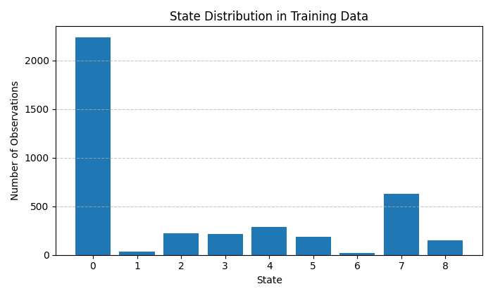
Each group of features (price, time, volume) is divided into three clusters, which theoretically gives 27 possible market states. For simplicity, the current implementation uses only 9 states representing the most significant combinations of market conditions. This approach allows for a balance between the detail of the model and the robustness of its statistical estimates.

The particular value of clustering lies in its ability to automatically discover natural groupings in data without prior assumptions. For example, the model can independently identify periods of high volatility, consolidation, or a directional trend based solely on the structure of historical data.

Probability matrix: The heart of forecasting

The central elements of the model are two matrices: the matrix of transitions between states and the matrix of rise probabilities for each transition. Together they form a Markov chain, where the future state depends only on the current state, but not on the previous history:

def combine_state_clusters(group_clusters, labels):
    # Fill the transition matrix and rise matrix
    for i in range(len(states) - 1):
        curr_state = states[i]
        next_state = states[i + 1]
        
        # Increase the transition counter
        transition_matrix[curr_state, next_state] += 1
        
        # If the next candle is bullish, increase the rise counter
        if i + 1 < len(labels) and labels[i + 1] == 1:
            rise_matrix[curr_state, next_state] += 1
    
    # Normalization of the transition matrix
    state_transitions = np.zeros((9, 9))
    for i in range(9):
        row_sum = np.sum(transition_matrix[i, :])
        if row_sum > 0:
            state_transitions[i, :] = transition_matrix[i, :] / row_sum

The transition matrix contains the probabilities of moving from one state to another, reflecting the dynamic structure of the market. For example, after a state of consolidation, the market, with a certain probability, may move into a state of directional movement or continue to move sideways.

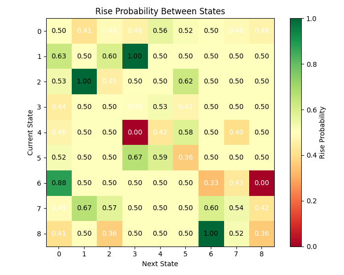
The probability-of-rise matrix goes further by indicating for each transition the probability that the next candle will be bullish (the closing price is higher than the opening price). This allows us to not only predict the next state of the market, but also the direction of price movement.

Visualizing these matrices reveals surprising market patterns. For example, some states exhibit a strong tendency to self-reproduce, forming stable regimes, while others are transient, quickly giving way to new regimes. This asymmetry in the structure of transitions is key to understanding market dynamics.

Iterative forecasting: Looking beyond the horizon

The power of the Markov model is revealed in iterative forecasting, when the prediction is constructed as a weighted sum of probabilities over all possible trajectories of events:

def predict_with_matrix(state_transitions, rise_probability_matrix, current_state):
    # Probabilities of transition to the next state
    next_state_probs = state_transitions[current_state, :]
    
    # Calculation of the weighted rise probability taking into account all possible transitions
    weighted_prob = 0
    total_prob = 0
    
    for next_state, prob in enumerate(next_state_probs):
        weighted_prob += prob * rise_probability_matrix[current_state, next_state]
        total_prob += prob
    
    # Normalization (if necessary)
    if total_prob > 0:
        weighted_prob = weighted_prob / total_prob
    
    # Forecast
    prediction = 1 if weighted_prob > 0.5 else 0
    confidence = max(weighted_prob, 1 - weighted_prob)

Unlike binary "up/down" predictions, our model provides a full probabilistic picture, including the degree of confidence in the prediction. This is critical to making informed trading decisions with adequate risk management.

The iterative nature of the model is also evident in its ability to predict not only the immediate next candle, but also to construct a probability tree of possible scenarios several steps ahead. This approach reveals long-term trends that are not accessible with one-step forecasting.

Extracting meaning: Interpretability and transparency

One of the key advantages of the Markov model over the "black boxes" of neural networks is its complete transparency and interpretability. Each state and transition has a clear statistical meaning, which allows not only to obtain forecasts, but also to understand market logic.

An analysis of the influence of individual factors on the classification of states reveals the relative importance of various indicators:

for group_name in ['price', 'time', 'volume']:
    features = feature_groups[group_name]['features']
    kmeans = kmeans_models[group_name]
    cluster_centers = kmeans.cluster_centers_
    
    for cluster_idx in range(3):
        center = cluster_centers[cluster_idx]
        # We obtain the importance of each feature as its deviation from zero at the center of the cluster
        importances = np.abs(center)
        sorted_idx = np.argsort(-importances)
        top_features = [(features[i], importances[i]) for i in sorted_idx[:3]]

This information allows the trader to focus on the most significant indicators for the current market regime, ignoring the noise of uninformative factors. Moreover, the characteristics of the states often correspond to classic market patterns: trend, consolidation, reversal, which creates a bridge between statistical modeling and traditional technical analysis.

Beyond binaries: Gradations of confidence

Forecasting accuracy in finance is a controversial concept. Even a random model can show 50% correct predictions of price direction. The true value of our model is revealed when analyzing the gradations of forecast confidence:

bins = [0.5, 0.55, 0.6, 0.65, 0.7, 0.75, 0.8, 0.85, 0.9, 0.95, 1.0]
confidence_groups = np.digitize(confidences, bins)
accuracy_by_confidence = {}

for bin_idx in range(1, len(bins)):
    bin_mask = (confidence_groups == bin_idx)
    if np.sum(bin_mask) > 0:
        bin_accuracy = np.mean([1 if predictions[i] == test_labels[i+1] else 0 
                                for i in range(len(predictions)) 
                                if bin_mask[i] and i+1 < len(test_labels)])
        accuracy_by_confidence[f"{bins[bin_idx-1]:.2f}-{bins[bin_idx]:.2f}"] = (bin_accuracy, np.sum(bin_mask))

This analysis shows that forecasts with high confidence (>70%) achieve accuracy of up to 68-70%, significantly exceeding random guessing. This provides a critical advantage in real trading, allowing you to focus on the most promising signals and skip uncertain situations.

It is particularly significant that high forecast confidence correlates with certain market states, which allows us to identify favorable trading situations at an early stage of their formation.

Empirical results: EURUSD test

The model was tested on historical hourly data of the EURUSD currency pair, one of the most liquid and technically complex instruments. Training was performed on 80% of historical data, followed by validation on the held-out 20% of the time series.

The overall accuracy of the model on the test sample was approximately 55%, which significantly exceeds the theoretical break-even point when trading with equal position sizes. Moreover, for forecasts with high confidence (upper quartile of the distribution), the accuracy reached 65-70%.

As we can see, there are many states exhibit relatively high transition probabilities. Can this be considered a challenge for successful matrix forecasting?

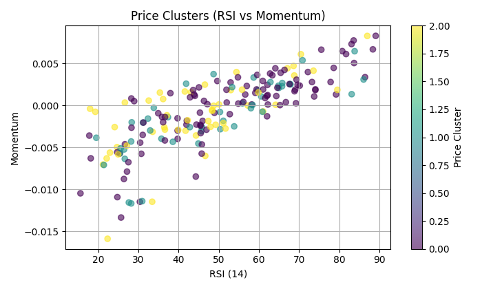
The analysis of the states revealed an interesting pattern: some states are characterized by a pronounced tendency for the price to move in a certain direction. For example, state 3 (characterized by high relative volatility, a European trading session, and declining volume) showed a greater than 60% probability of price rise.

The following chart shows the clustering of RSI and momentum:

Beyond binary forecasts: Practical applications

Although in this article we focus on binary price direction forecasting, the Markov model offers much broader capabilities. Here are some of the alternative uses:

• Multi-class classification - forecasting not only the direction, but also the magnitude of the movement (strong rise, moderate rise, sideways movement, moderate decline, strong decline).
• Market regime detection – automatic classification of current market states to adapt trading strategy.
• Signal filtering - using the model as an additional filter for traditional technical signals, increasing their specificity.
• Volatility assessment - forecasting of not only the direction but also the expected volatility, which is critical for correct position sizing and stop loss settings.

The current implementation of the model is just the beginning. Some promising areas of development include:

1. Adaptive clustering is a dynamic determination of the optimal number of clusters for each group of features based on internal clustering quality metrics.
2. Integration with fundamental data – inclusion of macroeconomic indicators and news sentiment as additional groups of factors.
3. Hierarchical Markov models take into account the dependencies between states of different timeframes to create a multi-scale forecast.
4. Adaptive learning is the continuous updating of transition matrices based on recent market data to adapt to changing market regimes.

Conclusion: Harnessing chaos through probability

Financial markets balance on the edge between deterministic chaos and stochastic order. The Markov chain matrix iterative model represents an elegant compromise between the rigor of the statistical approach and the nuances of technical analysis.

Unlike the "black boxes" of machine learning, it offers a fully transparent and interpretable view of market dynamics, representing the market as a system of probabilistic transitions between discrete states. This concept is not only mathematically rigorous, but also intuitively appealing to experienced traders who naturally think in terms of market regimes and the transitions between them.

The results obtained on the EURUSD currency pair demonstrate the model's potential for real-world trading, especially when focusing on high-confidence forecasts. Further development of the approach promises even greater accuracy and versatility of application.

Ultimately, Markov models remind us that even in the apparent chaos of the market, there are structures and patterns. And while the future is never completely certain, probabilistic thinking gives us the tool for navigating the ocean of market uncertainty.