Price Movement: Mathematical Models and Technical Analysis

Introduction

Being the largest financial market, Forex attracts a huge number of traders seeking to profit from exchange rate fluctuations. However, market volatility and unpredictability make it very difficult to predict price movements. Therefore, the development and application of effective forecasting models is one of the main tasks for a trader.

Despite the apparent randomness, price movements on the foreign exchange market are subject to certain patterns. However, effective forecasting remains a challenging task. Mathematical models based on statistical analysis seek to identify these patterns in historical data and build formal algorithms capable of predicting price movements. These models (which can be roughly divided into "complex" and "very complex") allow you to assess the likelihood of various scenarios and make informed trading decisions.

On the other hand, technical analysis, which relies on graphical analysis and the use of indicators, offers a more intuitive approach to forecasting. Traders study price charts, identify support and resistance levels, and use various indicators to make trading decisions.

This article examines both mathematical models and technical analysis methods used to predict price movements. We will look at various approaches, their advantages and disadvantages, and discuss the possibilities of combining them to improve the efficiency of trading strategies. Understanding how mathematical models and technical analysis methods work can help you improve your trading efficiency, reducing the risk of losses and increasing the likelihood of successful trades.

Simple models

Let's look at a trading strategy with these rules:

• when a new bar opens, the previously opened position is closed and a new one is opened;
• the direction of the opened position is determined randomly.

You might ask, "So, what's new here"? The new thing is that I have suddenly become a fan of the efficient-market hypothesis. If you also become a fan of this hypothesis, then you too will argue that predicting price movements is pointless. Prices move wherever and however they want. The market has some complete information, in accordance with which price changes occur. The trader does not have such information, and he can only hope that his decision will align with the market direction.

Let's try this strategy. The only configurable parameter is the initialization number of the random number generator. By changing this parameter, we can select the desired sequence of trades.

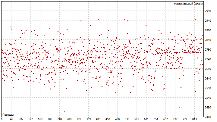
As you can see, in 800 optimizer passes, there is not even a hint of profitability. This result may be due to the influence of the spread. Due to the spread, the difference between the open and close prices of positions may even be negative. To avoid this, we might want to switch to some higher timeframe. But such a transition is equivalent to increasing the time it takes to hold a position. Let's take into account the obtained results and make several adjustments to the trading strategy:

• the position direction remains random;
• the position holding time is set by a trader;
• a new position opens if there are no other positions;
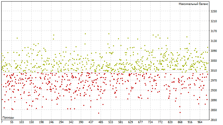
• positions are closed using stop orders.

I took the stop loss and take profit values from this article. The parameter being optimized remains the same. Apparently, the changes have benefited the strategy. We have some winning options.

In general, to find the best initializing number, you can use the secretary problem. Let us have N different options. Then the number of options that should be checked can be found using the equation:

In this case, we will get the following value:

We remember the option with the best result and continue to explore the remaining options. If a better result than the saved one appears, then further searching can be stopped. With a very high probability, we have found the best option of all possible ones.

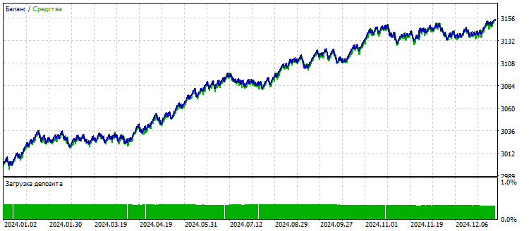
The only drawback of this algorithm is that its implementation can be very time-consuming. However, if you want to fully unlock the potential of this strategy, you will have to use this algorithm. I just picked the best option after 1000 passes. The results look good.

Until now, we have chosen the type of position to open randomly. What if there are some patterns in price movements that can help in this choice? Let's try to use a naive forecasting method. This forecast can be formulated as follows: the past defines the future. It is sufficient to look at any chart to understand that this method does not work. Let me change this forecast method a little: the next price will be the same as the current one plus an error:

With this approach, the main factor influencing the forecast is not the price, but the error. I use the term "error" because of the choice of forecasting model. But it can be replaced with "price increase". The term has changed, but the essence remains the same. Let's look at the statistics of these increments.

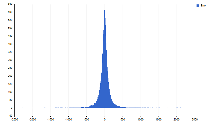
Looks like Laplace distribution. When studying financial time series, many researchers try to explain the obtained results using classical distributions. This approach is very convenient. The properties of these distributions are known, and modeling time series using them is not difficult. But it is not that simple. Classical distributions are mathematical abstractions that are almost never encountered in reality.

The distribution of real price values is what really important for a trader. Such distributions are called "empirical". They are obtained from observations, not from any theoretical assumptions. So, we have an empirical distribution of price increments. Let's discard the third of the smallest and largest increments. Then we will have a channel we can use to predict the future price value.

Note that we only need the current price to make a forecast. This model can be made more flexible. But to achieve this, we will have to resort to significant complications. If you are interested, please write in the comments. In the meantime, we are moving on to more complex models.

Linear trend

All traders love trends. Especially if the directions of a position and a trend coincide. A linear trend is defined by a simple equation:

This equation uses time as the independent variable. MetaQuotes proposes to count time from January 1, 1970. What if they are wrong? Maybe we should have started counting time from February 29th? Let's try to get rid of this shortcoming and find the most accurate beginning of time.

The linear trend equations for two consecutive bars look like this:

Now, let's find the differences between these equations:

If we simplify this equation, we get the following expression:

It is more convenient to express the difference in time as the number of bars between price readings. Then the equation becomes even simpler:

Please note that one of the trend parameters and time are no longer needed. The value of the next price can be obtained by adding the current price and the trend rate. After simplification, difficulties begin. We can define the parameters of the trend using, for example, the least squares method. But another approach can be used.

Let's assume that we already know the trend rate. Then, when a new price appears, we will adjust the trend rate according to the following rule: the forecast error and the change in trend rate should tend to zero. This rule can be set in another way: the trend rate should be stable over a fairly long period of time. The equation will look like this:

As a result, we get the following equation for calculating the updated value of the trend rate:

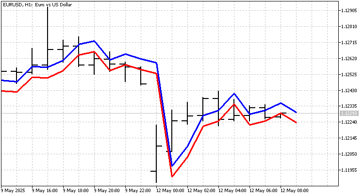
To recognize the presence of a trend, there should be a directional price movement over a number of bars. In this case, we obtain several equations of the form:

If we combine these equations into one, the speed of the trend will be measured relative to the average price value, which can be obtained using SMA. And the trend rate equation will take its final form:

The indicator built using this equation looks like this:

A simple trading strategy can be created based on this indicator. Opening and closing of positions will occur when the sign of the indicator values changes.

We have obtained some results, but the indicator itself requires further study and refinement. The change in trend rate can also be subject to its own trend. And these trends also need to be highlighted. The sum of such trends (if they really exist) will allow us to obtain more accurate signals.

Moving along the chart

One of the interesting models is related to random walk. If the price movement is random, then the distance traveled by the price and the time are related to each other as follows:

Let's make the assumption that we might have any time exponent. In other words, the price movement is subject to the following pattern:

Let's look at an algorithm that can be used to calculate the time exponent and the proportionality ratio. First, we need to set the N indicator period. With time, everything is simple - it is defined by non-negative integers starting from 1 to N. The traveled distance requires some more effort. The distance traveled by a price can be calculated by adding the absolute values of the differences between two consecutive prices:

In this case, the distance traveled should be calculated from the past to the future, summing the new values with the previous ones. It looks like this:

Now, we need to normalize the obtained distances. To do this, all values should be divided by the smallest distance traveled R[N-1].

Thus, we measure not the real distance, but the relative one. There is very little left to do - we need to take the logarithm of the obtained numbers. Moreover, we should take the logarithm of both the paths and the time.

Note that the logarithms of the oldest distance and time values are 0. They do not affect further calculations in any way. Taking this into account, the exponent and the proportionality ratio can be found using the equations:

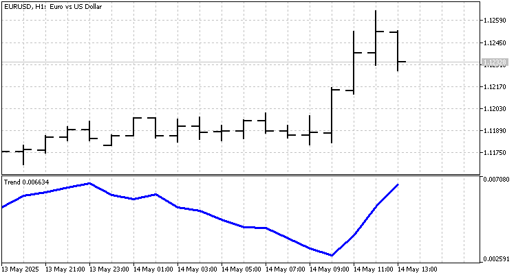
Now, let's look at how the exponent changes throughout history.

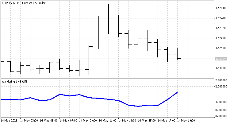
This parameter can be used to evaluate the nature of price movement. If it is close to 0, this indicates a weak price change - a flat. For a linear trend, this indicator is equal to 1. The exponent varies over a very wide range from 0 to approximately 2.5. Because of this, indicators that prioritize recent price values become important. Such indicators include the well-known EMA and LWMA.

We will try to develop an indicator whose weights are determined using figurative numbers. Let L be the level of a number. Then the n th polygonal number can be calculated using the equation:

These numbers serve as the indicator’s weights. Such an indicator will react to price changes faster than LWMA. But its "memory" is longer than that of EMA, so it will smooth the time series better.

Let's test this indicator using a simple strategy that generates signals when the price crosses the indicator line.

The test results are not impressive. But it is important to remember that a large number of indicators can be built based on figurative numbers, each of which will respond to its own trend. If the signals from each indicator are processed separately, the results can be pleasantly surprising.

Conclusion

In this article, we examined various approaches to describing and forecasting price movements in the Forex market. Even a simple strategy based on randomly choosing a position direction can be profitable with proper optimization of parameters, such as position holding time and stop-loss and take-profit levels. This emphasizes the importance of risk management and adapting to market conditions. 

The variety of approaches to forecasting Forex price movements highlights the importance of choosing the appropriate model based on specific market conditions and the trader's goals. Further research and development in this area could lead to the creation of even more efficient and reliable forecasting models, allowing traders to make more informed decisions and increase their profitability.

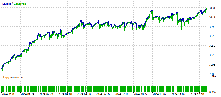
The following programs were used in writing this article.

Name	Type	Management
EA Picky Bride	EA	Seed - initializing number; Duration - expected position holding time, not less than 1.
Error	script	Duration - number of bars the price increment is calculated for, not less than 1; ScreenShot - when enabled, the script saves the image in the Files folder.
Price Increments	indicator	Percent - percentage of the largest and smallest values to discard when constructing a forecast. Valid values are 1 - 99.
Trend	indicator	iPeriod - indicator period, not less than 1.
EA Trend	EA
Wandering	indicator	iPeriod - indicator period, not less than 3.
Figurative Numbers	indicator	iPeriod - indicator period, not less than 2. Lvl - figurative number type. 1 - SMA, 2 - LWMA, then come the classic figurative numbers.
EA Figurative Numbers	EA