
CFTC Data Mining in Python and Building an AI Model

The Forex market is the largest in the world, but its high volatility makes forecasting difficult. COT/TFF reports provide insight into the actions of smart money and help uncover hidden market trends.
The proposed approach combines COT/TFF data and market quotes into a single Python model with automated trading via MetaTrader 5. This allows us to move from analysis to action without delays and human intervention.
Theoretical basis
What are COT and TFF reports?
Imagine having the opportunity to look into the portfolios of the largest players in the foreign exchange market – hedge funds with billions in assets, pension funds, investment banks. This is exactly what the COT and TFF reports, published every Friday by the US Commodity Futures Trading Commission (CFTC), do.
These reports emerged after the market crises of the 1970s and 1980s, when regulators realized that market participants needed information about what major players were doing. Now everyone who holds positions above a certain threshold is required to disclose their positions. The CFTC collects this information and publishes it in aggregate form, showing positions as of the end of Tuesday.
Who's who in the market: Participants and their motivations
Commercial traders — real business that uses futures not for speculation, but to protect against risks. An airline buys oil futures to lock in the price of fuel. An exporter sells currency futures to protect against a fall in the exchange rate. A farmer sells wheat futures in advance to know how much they will receive for the harvest.
Non-commercial traders — speculators who trade to profit from price movements. Hedge funds, investment banks, large management companies. They are often referred to as "smart money" because they have the resources to deeply analyze the markets.
Small traders — all other participants with positions below the reporting thresholds. Retail traders, small funds, individual speculators.
What do the COT reports show?
COT reports provide an overall picture of all futures markets. For each participant group, long positions (bets on the rise), short positions (bets on the fall), and net positions (the difference between long and short) are shown. Open interest shows the total number of active contracts in the market.
For example, if non-commercial traders are net long EUR by +120,000 contracts, this means that speculators are generally betting on EURUSD to rise. If commercial traders show -115,000 contracts, then hedgers are either expecting EUR to weaken or are simply protecting themselves from currency risks.
What do TFF reports add?
TFF reports focus only on financial futures and provide a more detailed picture of institutional positions. Here, non-commercial traders are divided into subcategories: leveraged funds (aggressive hedge funds that heavily use borrowed funds) and asset managers (conservative pension funds and insurance companies). There are also dealers and intermediaries – banks that provide market liquidity.
This detail is critical. If leveraged funds sharply increase their long USD positions, it is a signal of short-term speculative interest. If asset managers do the same, it indicates a long-term shift in institutional investor sentiment.
Why do traders need this?
The main value of the reports is that they show where the smart money is moving before it is reflected in prices. Large players often act based on data unavailable to ordinary market participants.
Identification of extremes. When speculators take record long positions, the market is often overbought and ready for a correction. The opposite situation signals a possible rebound. It works on the principle of contrarian trading - acting against the crowd in moments of extremes.
Confirmation of trends. If the price rises and non-commercial traders continue to increase their long positions, the trend is strong. If they start reducing positions when prices rise, the trend weakens.
Early detection of reversals. Divergences between price and positions often precede reversals. The price may continue to rise, but if major players are already reducing bullish exposure, a reversal is near.
Practical example
Let's say the EURUSD report shows that leveraged funds hold +85,000 contracts, asset managers +25,000, and dealers -95,000. This means that both aggressive speculators and conservative institutional investors are betting on EUR rise. Dealers take the opposite side, perhaps servicing client orders or hedging their own risks. The overall signal is bullish for EUR.
Important nuances
The data is published with a three-day delay, which is critical in rapidly changing markets. Not all commercial positions are pure hedging — some banks may speculate under the guise of commercial activity. Algorithmic trading and machine learning are changing traditional behavioral patterns of participants.
Modern algorithms can use the COT/TFF reports themselves to make decisions, which creates self-fulfilling prophecies and complicates data interpretation.
Why does this work?
The COT and TFF reports work because they show real money positions, not opinions or forecasts. When a hedge fund bets billions of dollars on a particular market direction, it is a far more significant signal than any public comment. This data reflects the collective wisdom of the most informed and resourced market participants.
When combined with machine learning and automated trading, institutional position analysis becomes a powerful tool for creating trading strategies based on the behavior of those who really move the markets.
Price forecasting using COT/TFF data
Price forecasting is based on the assumption that the positions of major players are correlated with future price movements. For example, an increase in long positions by non-commercial traders may signal a bullish market, while an increase in short positions may indicate bearish sentiment. This data is used as features for a machine learning model, supplemented with historical prices from MetaTrader 5 and technical indicators such as volatility and moving averages. This approach allows us to capture complex relationships between market sentiment and price trends.
Data preparation
COT and TFF reports are published in Excel format on the CFTC website. The requests library is used to load them, and pandas is used for processing. The code below demonstrates loading and preprocessing COT data with caching to improve performance:
import requests
import zipfile
import pandas as pd
import os
import logging
import MetaTrader5 as mt5
from datetime import datetime, timedelta
import matplotlib.pyplot as plt
import seaborn as sns
from sklearn.ensemble import RandomForestRegressor
from sklearn.preprocessing import StandardScaler
from sklearn.model_selection import train_test_split
import importlib.util
import glob
import asyncio

logging.basicConfig(level=logging.DEBUG, format='%(asctime)s - %(levelname)s - %(message)s')
logger = logging.getLogger(__name__)

plt.style.use('ggplot')
plt.rcParams['figure.figsize'] = [10, 6]

COT_URL = "https://www.cftc.gov/files/dea/history/dea_fut_xls_2024.zip"
TFF_URL = "https://www.cftc.gov/files/dea/history/fut_fin_xls_2024.zip"
OUTPUT_DIR = "data"
os.makedirs(OUTPUT_DIR, exist_ok=True)

def load_cot_reports() -> pd.DataFrame:
    cache_path = os.path.join(OUTPUT_DIR, "cot_report.csv")
    if os.path.exists(cache_path):
        logger.info(f"Loading COT data from cache: {cache_path}")
        return pd.read_csv(cache_path)

    try:
        response = requests.get(COT_URL)
        response.raise_for_status()
        zip_path = os.path.join(OUTPUT_DIR, "cot_data.zip")
        with open(zip_path, "wb") as f:
            f.write(response.content)

        with zipfile.ZipFile(zip_path, 'r') as zip_ref:
            zip_ref.extractall(OUTPUT_DIR)
            excel_file = [f for f in zip_ref.namelist() if f.endswith('.xls') or f.endswith('.xlsx')][0]

        cot_data = pd.read_excel(os.path.join(OUTPUT_DIR, excel_file))
        relevant_columns = [
            "Market_and_Exchange_Names",
            "NonComm_Positions_Long_All",
            "NonComm_Positions_Short_All",
            "Comm_Positions_Long_All",
            "Comm_Positions_Short_All",
            "Open_Interest_All"
        ]
        cot_data = cot_data[relevant_columns]
        cot_data["Net_NonComm"] = cot_data["NonComm_Positions_Long_All"] - cot_data["NonComm_Positions_Short_All"]
        cot_data["Net_Comm"] = cot_data["Comm_Positions_Long_All"] - cot_data["Comm_Positions_Short_All"]
        cot_data.to_csv(cache_path, index=False)
        logger.info(f"COT report saved in {cache_path}")
        return cot_data
    except Exception as e:
        logger.error(f"Error loading COT data: {e}")
        return pd.DataFrame()
A similar process is used for TFF reports, filtering by currency futures and calculating net positions for leveraged funds and asset managers. Data caching minimizes network requests, speeding up reprocessing.
Integration with MetaTrader 5
Historical prices are downloaded via the MetaTrader 5 library, which provides access to market data. The code below gets hourly prices for the last 30 days:
def get_historical_prices(pair: str, days_history: int = 30) -> pd.DataFrame:
    if not mt5.initialize():
        logger.error("MT5 initialization failed")
        return pd.DataFrame()

    timeframe = mt5.TIMEFRAME_H1
    utc_from = datetime.now() - timedelta(days=days_history)
    rates = mt5.copy_rates_from(pair, timeframe, utc_from, 24 * days_history)

    if rates is None or len(rates) == 0:
        logger.warning(f"No historical data for {pair}")
        return pd.DataFrame()

    df = pd.DataFrame(rates)
    df['time'] = pd.to_datetime(df['time'], unit='s')
    df.set_index('time', inplace=True)
    df['price_change_24h'] = df['close'].shift(-24) / df['close'] - 1
    df.dropna(inplace=True)
    return df[['open', 'high', 'low', 'close', 'tick_volume', 'price_change_24h']]
Data processing and merging
COT, TFF, and historical price data are combined, and derived features are added: volatility (the difference between the high and low prices, normalized to the closing price), 24-hour moving averages for volume and price, and lags and percentage changes for COT and TFF positions.
Feature preparation code:
def prepare_features(pair: str, cot_data: pd.DataFrame, tff_data: pd.DataFrame) -> pd.DataFrame:
    df_prices = get_historical_prices(pair)
    if df_prices.empty:
        logger.warning(f"No price data available for {pair}")
        df = pd.DataFrame(index=[datetime.now()], columns=['close', 'price_change_24h'])
        df['close'] = 1.0
        df['price_change_24h'] = 0.0
    else:
        df = df_prices.copy()

    df['volatility'] = (df['high'] - df['low']) / df['close']
    df['volume_sma_24'] = df['tick_volume'].rolling(window=24).mean()
    df['price_sma_24'] = df['close'].rolling(window=24).mean()
    df['price_change_1h'] = df['close'].pct_change()

    market = map_pair_to_cot_tff(pair)
    if market and not cot_data.empty:
        cot_subset = cot_data[cot_data["Market_and_Exchange_Names"].str.contains(market, case=False, na=False)]
        if not cot_subset.empty:
            cot_features = cot_subset[['Net_NonComm', 'Net_Comm']].mean().to_frame().T
            for col in cot_features.columns:
                df[col] = cot_features[col].iloc[0]

    if market and not tff_data.empty:
        tff_subset = tff_data[tff_data["Market_and_Exchange_Names"].str.contains(market, case=False, na=False)]
        if not tff_subset.empty:
            tff_features = tff_subset[['Net_Lev_Money', 'Net_Asset_Mgr']].mean().to_frame().T
            for col in tff_features.columns:
                df[col] = tff_features[col].iloc[0]

    for col in ['Net_NonComm', 'Net_Comm', 'Net_Lev_Money', 'Net_Asset_Mgr']:
        if col in df.columns:
            df[f'{col}_lag1'] = df[col].shift(1)
            df[f'{col}_change'] = df[col].pct_change().fillna(0)

    df.dropna(inplace=True)
    return df

def map_pair_to_cot_tff(pair: str) -> str:
    mapping = {
        'EURUSD': 'EURO FX',
        'GBPUSD': 'BRITISH POUND',
        'USDJPY': 'JAPANESE YEN',
        'AUDUSD': 'AUSTRALIAN DOLLAR',
        'USDCAD': 'CANADIAN DOLLAR',
        'USDCHF': 'SWISS FRANC',
        'NZDUSD': 'NEW ZEALAND DOLLAR'
    }
    base_pair = pair.replace('.ecn', '')[:6]
    return mapping.get(base_pair, '')
To improve accuracy, hyperparameters such as the number of trees or maximum depth can be optimized, and cross-validation can be used to assess the robustness of the model. The feature importance is saved in a CSV file to analyze their impact on forecasts.
Forecasting and visualization
Price forecasting
The forecast is made based on the latest data, predicting the percentage change in price in 24 hours, which is applied to the current market price. Forecast code:
async def get_price_forecast(pair: str, model, scaler) -> dict:
    df = prepare_features(pair, cot_data, tff_data)
    if df.empty:
        logger.warning(f"No data to forecast for {pair}")
        return {'pair': pair, 'forecast_price': None, 'confidence': 0.0}

    X_latest = df.drop(columns=['price_change_24h']).iloc[-1:]
    X_scaled = scaler.transform(X_latest)

    price_change_pred = model.predict(X_scaled)[0]
    confidence = model.score(X_scaled, df['price_change_24h'].iloc[-1:]) if len(df) > 1 else 0.6

    tick = mt5.symbol_info_tick(pair)
    if not tick:
        logger.warning(f"No current data for {pair}")
        return {'pair': pair, 'forecast_price': None, 'confidence': 0.0}

    current_price = (tick.bid + tick.ask) / 2
    forecast_price = current_price * (1 + price_change_pred)

    forecast_df = pd.DataFrame([{
        'forecast_price': forecast_price,
        'confidence': confidence,
        'current_price': current_price,
        'price_change_pred': price_change_pred,
        'timestamp': datetime.now()
    }])
    output_path = os.path.join(OUTPUT_DIR, f"forecast_{pair}.csv")
    forecast_df.to_csv(output_path, index=False)
    logger.info(f"Forecast for {pair} saved in {output_path}")

    visualize_forecast(pair, current_price, forecast_price, confidence)

    return {
        'pair': pair,
        'forecast_price': forecast_price,
        'confidence': max(0.0, min(1.0, confidence))
    }
Visualization of results
For analysis, charts of the current and projected price, as well as net COT and TFF positions, are created. Visualization code:
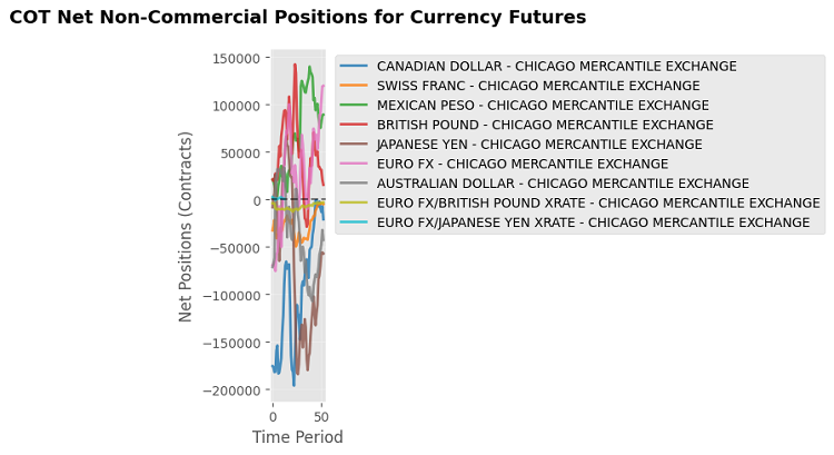
def visualize_cot_data(cot_data: pd.DataFrame):
    if cot_data.empty or "Net_NonComm" not in cot_data.columns:
        logger.warning("No COT data available for visualization")
        return

    plt.figure(figsize=(14, 8))
    for market in cot_data["Market_and_Exchange_Names"].unique():
        market_data = cot_data[cot_data["Market_and_Exchange_Names"] == market]
        plt.plot(range(len(market_data)), market_data["Net_NonComm"], label=market, alpha=0.7)

    plt.title("Net Non-Commercial positions for currency futures")
    plt.xlabel("Entry")
    plt.ylabel("Net positions")
    plt.legend()
    plt.grid(True, alpha=0.3)
    plt.tight_layout()
    output_path = os.path.join(OUTPUT_DIR, "cot_net_positions.png")
    plt.savefig(output_path, dpi=150)
    plt.close()
    logger.info(f"Chart of net COT positions saved in {output_path}")

def visualize_tff_data(tff_data: pd.DataFrame):
    if tff_data.empty or "Net_Lev_Money" not in tff_data.columns:
        logger.warning("No TFF data available for visualization")
        return

    plt.figure(figsize=(14, 8))
    for market in tff_data["Market_and_Exchange_Names"].unique():
        market_data = tff_data[tff_data["Market_and_Exchange_Names"] == market]
        plt.plot(range(len(market_data)), market_data["Net_Lev_Money"], label=market, alpha=0.7)

    plt.title("Leveraged Funds net positions for currency futures (TFF)")
    plt.xlabel("Entry")
    plt.ylabel("Net positions")
    plt.legend()
    plt.grid(True, alpha=0.3)
    plt.tight_layout()
    output_path = os.path.join(OUTPUT_DIR, "tff_net_positions.png")
    plt.savefig(output_path, dpi=150)
    plt.close()
    logger.info(f"Chart of net TFF positions saved in {output_path}")

def visualize_forecast(pair: str, current_price: float, forecast_price: float, confidence: float):
    plt.figure(figsize=(8, 5))
    plt.bar(['Current Price', 'Forecast Price'], [current_price, forecast_price], color=['blue', 'green'], alpha=0.7)
    plt.title(f"Price forecast in 24 hours for {pair} (Confidence: {confidence:.2f})")
    plt.ylabel('Price')
    plt.tight_layout()
    output_path = os.path.join(OUTPUT_DIR, f"forecast_{pair}_plot.png")
    plt.savefig(output_path, dpi=150)
    plt.close()
    logger.info(f"Forecast graph saved to {output_path}")
Graphs help visually assess market sentiment and forecast accuracy by providing traders with a clear understanding of the data.
Optimization and error handling
Data caching
To minimize network requests, COT and TFF data are cached in CSV files, allowing for reuse of up-to-date data and faster handling. The cache is checked before loading new data, and only if it is missing or out of date is a new request made.
Checking dependencies
Before execution, the code checks whether the xlrd and openpyxl libraries are installed:
def check_dependencies():
    dependencies = ['xlrd', 'openpyxl']
    for dep in dependencies:
        if not importlib.util.find_spec(dep):
            logger.error(f"Missing dependency: {dep}. Install it using 'pip install {dep}'.")
            raise ImportError(f"Missing dependency: {dep}")
Error handling
The code includes exception handling for all critical operations: loading data, connecting to MetaTrader 5, and training the model. This ensures the system is resilient to failures, such as missing data or connection problems.
Practical use
Testing the model
To evaluate the model, it is recommended to test on historical data for 2024. R² metrics and feature importance are saved in CSV files for analysis. Testing allows us to evaluate the accuracy of forecasts and identify the most significant features, such as net positions of non-commercial traders or volatility.
Integration into a trading strategy
Forecasts can be used for automated trading via the MetaTrader 5 library. For example, if the predicted price change is more than 0.5% and the model has high confidence (above 0.7), you can open long or short positions. Code for automatic trading:
def execute_trade(pair: str, forecast_price: float, confidence: float):
    if not mt5.initialize():
        logger.error("MT5 initialization failed")
        return

    symbol_info = mt5.symbol_info(pair)
    if not symbol_info:
        logger.warning(f"{pair} symbol not found")
        return

    current_price = (mt5.symbol_info_tick(pair).bid + mt5.symbol_info_tick(pair).ask) / 2
    if confidence > 0.7 and forecast_price > current_price * 1.005:
        request = {
            "action": mt5.TRADE_ACTION_DEAL,
            "symbol": pair,
            "volume": 0.1,
            "type": mt5.ORDER_TYPE_BUY,
            "price": mt5.symbol_info_tick(pair).ask,
            "type_time": mt5.ORDER_TIME_GTC,
            "type_filling": mt5.ORDER_FILLING_IOC,
        }
        result = mt5.order_send(request)
        logger.info(f"Opened long position for {pair}: {result}")
    elif confidence > 0.7 and forecast_price < current_price * 0.995:
        request = {
            "action": mt5.TRADE_ACTION_DEAL,
            "symbol": pair,
            "volume": 0.1,
            "type": mt5.ORDER_TYPE_SELL,
            "price": mt5.symbol_info_tick(pair).bid,
            "type_time": mt5.ORDER_TIME_GTC,
            "type_filling": mt5.ORDER_FILLING_IOC,
        }
        result = mt5.order_send(request)
        logger.info(f"Opened short position for {pair}: {result}")
Expanding functionality
To improve the model, we can add technical indicators, such as RSI or MACD, to take into account additional market signals. Alternative algorithms, such as gradient boosting (XGBoost) or neural networks, can improve forecast accuracy. Dynamic updating of COT and TFF data can be implemented through a task scheduler, such as the 'schedule' library, to automatically retrieve new reports as they are published. It can also be extended to analyze other assets, such as commodities or indices, with appropriate adaptation of the features.
Full implementation: CurrencyForecastModule
For ease of integration, all functions are combined into the CurrencyForecastModule class, which encapsulates data loading, model training, forecasting, and visualization:
class CurrencyForecastModule:
    def __init__(self, pairs: list, days_history: int = 30):
        self.pairs = pairs
        self.days_history = days_history
        self.models = {}
        self.scalers = {}
        self.forecasts = {}

        check_dependencies()
        if not mt5.initialize():
            logger.error("MT5 initialization failed. Ensure MT5 terminal is running and connected.")
            raise RuntimeError("MT5 initialization failed")

        self._validate_symbols()
        self._initialize_data()

    def _validate_symbols(self):
        available_symbols = [s.name for s in mt5.symbols_get()]
        logger.info(f"Available symbols in MT5: {available_symbols}")
        self.symbol_mapping = {}
        for pair in self.pairs[:]:
            if pair in available_symbols:
                self.symbol_mapping[pair] = pair
            else:
                base_pair = pair.split('.')[0]
                if base_pair in available_symbols:
                    self.symbol_mapping[pair] = base_pair
                    logger.info(f"Matched: {pair} -> {base_pair}")
                else:
                    logger.warning(f"{pair} symbol not found in MT5. Skipped.")
                    self.pairs.remove(pair)

    def _initialize_data(self):
        logger.info("Initializing data for CurrencyForecastModule...")
        self.cot_data = load_cot_reports()
        self.tff_data = self._load_tff_reports()
        for pair in self.pairs:
            self._train_model(pair)

    def _load_tff_reports(self) -> pd.DataFrame:
        cache_path = os.path.join(OUTPUT_DIR, "tff_report.csv")
        if os.path.exists(cache_path):
            logger.info(f"Loading TFF data from cache: {cache_path}")
            return pd.read_csv(cache_path)

        try:
            response = requests.get(TFF_URL)
            response.raise_for_status()
            zip_path = os.path.join(OUTPUT_DIR, "tff_data.zip")
            with open(zip_path, "wb") as f:
                f.write(response.content)

            with zipfile.ZipFile(zip_path, 'r') as zip_ref:
                zip_ref.extractall(OUTPUT_DIR)
                logger.info(f"TFF archive contents: {zip_ref.namelist()}")

            excel_files = glob.glob(os.path.join(OUTPUT_DIR, "**", "*.xls*"), recursive=True)
            tff_files = [f for f in excel_files if 'FinFut' in f or 'fin' in f.lower()]
            if not tff_files:
                logger.error("TFF Excel file not found in extracted files")
                return pd.DataFrame()

            excel_file = tff_files[0]
            logger.info(f"Handling TFF file: {excel_file}")

            relevant_columns = [
                "Market_and_Exchange_Names",
                "Lev_Money_Positions_Long_All",
                "Lev_Money_Positions_Short_All",
                "Asset_Mgr_Positions_Long_All",
                "Asset_Mgr_Positions_Short_All",
                "Open_Interest_All"
            ]
            tff_data = pd.read_excel(excel_file, engine='xlrd' if excel_file.endswith('.xls') else 'openpyxl')
            available_columns = [col for col in relevant_columns if col in tff_data.columns]
            if not available_columns:
                logger.error("Expected columns in TFF data not found")
                return pd.DataFrame()

            tff_data = tff_data[available_columns]
            forex_markets = ["EURO FX", "JAPANESE YEN", "BRITISH POUND", "AUSTRALIAN DOLLAR",
                             "CANADIAN DOLLAR", "SWISS FRANC", "MEXICAN PESO", "NEW ZEALAND DOLLAR"]
            tff_data = tff_data[tff_data["Market_and_Exchange_Names"].str.contains('|'.join(forex_markets), case=False, na=False)]
            if "Lev_Money_Positions_Long_All" in tff_data.columns:
                tff_data["Net_Lev_Money"] = tff_data["Lev_Money_Positions_Long_All"] - tff_data["Lev_Money_Positions_Short_All"]
            if "Asset_Mgr_Positions_Long_All" in tff_data.columns:
                tff_data["Net_Asset_Mgr"] = tff_data["Asset_Mgr_Positions_Long_All"] - tff_data["Asset_Mgr_Positions_Short_All"]

            tff_data.to_csv(cache_path, index=False)
            logger.info(f"TFF report saved in {cache_path}")
            visualize_tff_data(tff_data)
            return tff_data
        except Exception as e:
            logger.error(f"Error loading TFF data: {e}")
            return pd.DataFrame()

    def _train_model(self, pair: str):
        df = prepare_features(pair, self.cot_data, self.tff_data)
        model, scaler = train_model(pair, df)
        if model and scaler:
            self.models[pair] = model
            self.scalers[pair] = scaler

    async def update_forecasts(self):
        logger.info("Updating price forecasts...")
        for pair in self.pairs:
            forecast = await get_price_forecast(pair, self.models.get(pair), self.scalers.get(pair))
            logger.info(f"Forecast for {pair}: Price={forecast['forecast_price']}, Confidence={forecast['confidence']:.2f}")

    def __del__(self):
        mt5.shutdown()
This class provides a modular structure for loading data, training models, and performing forecasts, simplifying integration into trading systems.
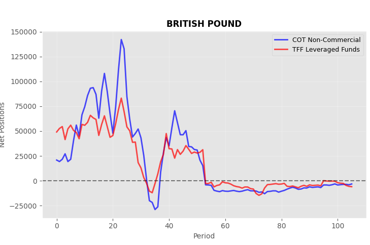
As a result, we receive forecasts and several graphs. Here, for example, is a chart of COT vs TFF positions:
The code ultimately produces 24-hour price forecasts for a group of symbols:
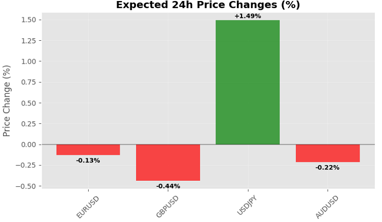
Although, of course, it would be more logical to use the Friday evening close as a forecast - then it will be consistent with the frequency of publication of the COT and TFF reports.
Conclusion
Using COT and TFF data with historical prices through the MetaTrader 5 Python library allows us to create efficient price forecasting models that can be integrated into trading strategies. The implemented solution automates data loading, model training, and trading execution, providing traders with a stable foundation for analysis and decision-making in financial markets. The code can be expanded by adding new indicators or algorithms, as well as automating data updates to ensure forecasts are always up-to-date.
Translated from Russian by MetaQuotes Ltd.
Original article: https://www.mql5.com/ru/articles/18303
Warning: All rights to these materials are reserved by MetaQuotes Ltd. Copying or reprinting of these materials in whole or in part is prohibited.
This article was written by a user of the site and reflects their personal views. MetaQuotes Ltd is not responsible for the accuracy of the information presented, nor for any consequences resulting from the use of the solutions, strategies or recommendations described.


| Net_NonComm,0.0,0.0. | |||
| Net_Comm,0.0,0.0. | |||
| Net_Lev_Money,0.0,0.0. | |||
| Net_Asset_Mgr,0.0,0.0 | |||
| Net_NonComm_lag1,0.0,0.0 | |||
| Net_NonComm_change,0.0,0.0 | |||
| Net_Comm_lag1,0.0,0.0 | |||
| Net_Comm_change,0.0,0.0 | |||
| Net_Lev_Money_lag1,0.0,0.0 | |||
| Net_Lev_Money_change,0.0,0.0 | |||
| Net_Asset_Mgr_lag1,0.0,0.0 | |||
| Net_Asset_Mgr_change,0.0,0.0 | |||
- Free trading apps
- Over 8,000 signals for copying
- Economic news for exploring financial markets
You agree to website policy and terms of use