Determining Fair Exchange Rates Using PPP and IMF Data

At some point, I realized I was spending more time searching for the "perfect" forecasting module than understanding what really drives exchange rates. So I asked myself a simple question: what if I put all those charts aside and tried to find the real value of a currency? Not the value the market happens to show at any given moment under the influence of emotion and speculation, but the one that follows from fundamental economic laws?

That question led me into several months of work. I started by studying purchasing power parity theory and ended up writing a full-fledged exchange rate analysis system in Python. This turned out to be much more interesting than any technical indicator.

Defining the problem

Forex market analysis often focuses on finding technical indicators and chart patterns, ignoring fundamental economic factors. A logical question arises: is it possible to determine the fair value of currencies based on economic laws, rather than short-term market sentiment and speculative movements?

This study presents a practical approach to solving this problem by creating a comprehensive system for calculating fair exchange rates based on purchasing power parity theory, implemented using the Python programming language.

Theoretical foundations of purchasing power parity
The classic example of McDonald's Big Mac demonstrates the essence of the theory: if a hamburger costs USD 5 in the US and EUR 9 in Europe, the fair exchange rate should be USD 1.8 per EUR. Behind this simple illustration lies a fundamental tool for analyzing currency markets that allows one to identify long-term imbalances beyond short-term market volatility.

The historical roots of the concept can be traced back to the 16th century, when Spanish traders observed price disparities between the metropolis and the colonies. If one peso bought a loaf of bread in Seville but three loaves in Mexico, this indicated a fundamental mismatch in the relative value of the currencies, requiring correction through a change in the exchange rate or price equalization.

PPP formulations
Absolute purchasing power parity asserts a direct relationship between exchange rates and the ratio of prices of identical goods in different countries. While theoretically elegant, this approach faces multiple distorting factors in practice: tax differences, regulatory barriers, transport costs, and trade restrictions.

S₁₂ = P₁ / P₂

where S₁₂ is the exchange rate of currency 1 to currency 2, P₁ and P₂ are the price levels in the respective countries.

Relative purchasing power parity focuses on the dynamics of price changes rather than on absolute levels. According to this formulation, if inflation in country A is 10% per annum and in country B it is 5%, country A's currency should weaken by 5% relative to country B's currency to maintain purchasing power parity.

S₁₂(t) / S₁₂(0) = [P₁(t) / P₁(0)] / [P₂(t) / P₂(0)]

Or in simplified form:

ΔS₁₂ = π₁ - π₂

where π₁, π₂ are the inflation rates in countries 1 and 2.

The relative approach was chosen as the methodological basis of the algorithm due to its greater practical applicability, better reflection of economic reality and the possibility of obtaining specific quantitative benchmarks for exchange rates.

Evaluation of available data sources

A study of existing PPP data providers revealed significant limitations for practical application. The OECD publishes official purchasing power parity rates with a lag of six months to a year. Data for 2023 only became available in mid-2024, which is unacceptable for dynamic foreign exchange markets.

Source	Refresh rate	Delay	Cost/year	Methodology transparency	Practical applicability
OECD	Annual	6-12 months	USD 0	Low	Research
Penn World Table	2-3 years	1-2 years	USD 0	Average	Academic
Bloomberg Terminal	Real-time	No	USD 24,000	None	Professional
Refinitiv Eikon	Real-time	No	USD 22,000	None	Professional

Penn World Table is updated at intervals of several years, with the latest available version containing information only up to 2019. While such a base is valuable for academic research, such time lags are critical for practical trading.

Bloomberg and Refinitiv commercial data providers offer more up-to-date information, but access costs start at USD 2,000 per month for the Bloomberg Terminal, with no guarantees of methodological transparency or data quality.

The problem of methodological opacity: A critical drawback of existing solutions is the lack of clarity in the computational procedures. The methodology for calculating OECD coefficients, the composition of consumer baskets, algorithms for processing statistical outliers and adjusting for qualitative differences in goods remain undocumented.

Large data providers operate as closed systems: the user receives numerical results without understanding their origin or the possibility of verification. This approach is unacceptable for serious financial analysis that requires complete control over computational processes.

Developing a custom system: : A decision was made to create an independent system for calculating PPP using publicly available data from international organizations — the International Monetary Fund, the World Bank, and national statistical services. The system must ensure complete transparency of algorithms and the ability to adapt the methodology to specific analytical tasks.

While development is significantly more complex than purchasing a ready-made solution, and requires learning multiple data sources, API formats, and statistical methods, this approach guarantees complete control over the calculation process and a deep understanding of the system's operation.

Architectural solution: A system of multiple methods

The fundamental problem with any PPP calculation is that there are multiple approaches to estimating a fair exchange rate, each with its own specific advantages and limitations. Choosing a single method inevitably leads to subjectivity of the results.

Data sources	PPP calculation methods	Results and signals
IMF API	Price Level	Fair rates
World Bank	GDP-Implied	Deviations from the market
National statistics	Inflation-Adjusted	Trading signals
Fallback data	Big Mac Proxy	Confidence indices
Market rates of currency pairs	Composite Method	Currency classification

The developed system uses several independent calculation methods in parallel with subsequent combination of results. Consistency between estimates from different methods increases confidence in the result, while significant differences indicate a high degree of uncertainty, which in itself provides valuable information about the state of the market.

The first approach is based on international price comparisons. The logic is simple: if a Swiss citizen spends one and a half times more on living than an American with the same standard of living, then the Swiss franc is overvalued by 50%.

I took the data for this method from international price comparison programs conducted under the auspices of the World Bank and the OECD. These programs compare the prices of standard consumer baskets in different countries and calculate relative price levels.

def _calculate_price_level_ppp(self) -> Dict:
    ppp_rates = {}
    for country, price_level in self.price_levels_2024.items():
        if country != 'US':
            ppp_factor = price_level / 100.0
            ppp_rates[country] = {
                'ppp_conversion_factor': ppp_factor,
                'price_level_index': price_level,
                'method': 'price_level_adjustment'
            }
    return ppp_rates

The advantage of this method is that it reflects real differences in the cost of living. The disadvantage is that the data is updated infrequently, once every few years.

The second approach is the one I came up with myself and I am still proud of it. The idea came to me while studying IMF data: what if we compare a country's GDP in national currency (from official statistics) with an estimate of the same GDP in USD (from international databases)?

The logic is this: if the Bank of Russia reports that Russia's GDP is RUB 150 trillion, and the World Bank estimates Russia's GDP at USD 2 trillion, then the implicit exchange rate is RUB 75 per USD. This is the rate, at which economies are valued "fairly" relative to each other.

def _calculate_gdp_implied_ppp(self, economic_data: pd.DataFrame):
    for country, gdp_usd_2023 in self.gdp_usd_estimates_2023.items():
        country_gdp_lcu = gdp_lcu_data[gdp_lcu_data['REF_AREA'] == country]
        if not country_gdp_lcu.empty:
            latest_data = country_gdp_lcu.sort_values('year').iloc[-1]
            gdp_lcu = latest_data['value']
            
            if gdp_lcu > 0:
                implied_rate = gdp_lcu / gdp_usd_2023

This method has proven to be surprisingly accurate and relevant. GDP data are updated quarterly, so the estimates are up-to-date. And since GDP is an aggregate measure of all economic activity, it reflects a currency's fundamental value well.

The third method implements the classic formula for relative PPP from textbooks. We take the historical exchange rate from some base point and adjust it for the accumulated difference in inflation between countries.

I chose 2020 as a baseline. It is recent enough to be relevant, but is still pre-pandemic to avoid distortions from extreme monetary policy.

def _calculate_inflation_adjusted_ppp(self, economic_data: pd.DataFrame):
    # Get the basic rate for 2020
    base_rate_2020 = GetBaseRate2020(base_currency, quote_currency)
    
    # Calculating the inflation differential
    inflation_differential = (base_data.inflation_rate - quote_data.inflation_rate) / 100.0
    
    # Adjust the base rate
    adjusted_rate = base_rate_2020 * (1 + inflation_differential)

The method is theoretically flawless and easy to explain. If inflation was higher in country A than in country B, then A's currency should weaken in proportion to this difference.

The only problem is the quality of inflation data. Different countries calculate inflation differently, and some tend to "embellish" the statistics. But overall, the method works well.

The fourth method is inspired by The Economist's famous Big Mac Index. The idea is that the Big Mac is a standardized product that is produced using the same technology all over the world. Its price should reflect the real differences in resource costs between countries.

The problem is that collecting current Big Mac prices is a separate research task. Instead, I use known data about relative price levels to model how much a standardized good should cost in each country.

def _calculate_big_mac_proxy_ppp(self):
    us_big_mac_price = 5.50
    for country, price_level in self.price_levels_2024.items():
        if country != 'US':
            local_big_mac_price = us_big_mac_price * (price_level / 100.0)
            ppp_rate = local_big_mac_price / us_big_mac_price

The method is not the most accurate, but it provides a good intuitive check on the results of other methods. If all other methods show that the currency is overvalued by 20%, and the "Big Mac method" gives a similar result, this increases confidence in the valuation.

The fifth method combines the results of all previous ones through weighted averaging. I spent a lot of time calibrating the weights, testing different combinations on historical data.

In the end, I settled on the following distribution:

• Price Level PPP: 30% (most fundamental)
• GDP-Implied PPP: 25% (most relevant)
• Inflation-Adjusted PPP: 25% (most theoretically sound)
• Big Mac Proxy: 20% (most intuitive)

def _calculate_composite_ppp(self, all_methods: Dict):
    weights = [0.30, 0.25, 0.25, 0.20]
    
    # Dynamic weight normalization
    if valid_methods < 4:
        total_weight = sum(weights[:valid_methods])
        normalized_weights = [w / total_weight for w in weights[:valid_methods]]
    
    composite_rate = sum(rate * weight for rate, weight in zip(rates, normalized_weights))

The key feature is dynamic normalization of weights. If some method cannot produce a result (for example, there is no inflation data), the weights of the remaining methods are increased proportionally. This is much smarter than simply eliminating "problematic" methods.

Program development

After months of theoretical preparation, it was time to take up the keyboard. I decided to write in Python — the language is fast enough for financial calculations, but also has excellent libraries for working with data.

The first and most important question is where to get the data? After reviewing dozens of sources, the choice fell on the International Monetary Fund API. Public, free, well documented and, most importantly, regularly updated.

def __init__(self):
    self.base_url = "http://dataservices.imf.org/REST/SDMX_JSON.svc"
    self.session = requests.Session()
    self.session.headers.update({
        'User-Agent': 'Manual-PPP-Calculator/1.0',
        'Accept': 'application/json'
    })

A small but important detail: I use requests.Session() instead of simple requests.get() calls. This allows for the reuse of TCP connections and significantly speeds up performance when making multiple requests to a single API.

User-Agent is not random either. Many APIs block requests without an explicit User-Agent or with the default value from Python. It is better to immediately introduce yourself as a serious application.

The next problem turned out to be more insidious than expected. Currency codes (USD, EUR, GBP) need to be somehow linked to country codes in the IMF system. This is where the surprises began.

EUR is not a country code, but a currency union code. In the IMF database, the Eurozone is designated as U2. Switzerland is CH, not SW. Great Britain is GB, not UK.

self.currency_country_map = {
    'USD': 'US', 'EUR': 'U2', 'GBP': 'GB', 'JPY': 'JP',
    'AUD': 'AU', 'CAD': 'CA', 'CHF': 'CH', 'NZD': 'NZ',
    'SEK': 'SE', 'NOK': 'NO', 'DKK': 'DK', 'PLN': 'PL'
}

It might seem like a small thing, but without proper mapping the whole system simply does not work. I spent a whole day debugging until I realized I was looking for data for non-existent country codes.

External APIs have a nasty habit of breaking at the most inopportune moments. The IMF API is no exception. Sometimes it is unavailable for several hours, sometimes it returns incomplete data, and sometimes it even returns an error for no apparent reason.

I decided to build a backup data system from the very beginning:

self.fallback_market_rates = {
    'EURUSD': 1.0850, 'GBPUSD': 1.2650, 'USDJPY': 148.50,
    'AUDUSD': 0.6750, 'USDCAD': 1.3550, 'USDCHF': 0.8850,
    'NZDUSD': 0.6150
}

self.price_levels_2024 = {
    'US': 100.0,    # Basic level
    'U2': 88.5,     # Eurozone is 11.5% cheaper than the US
    'GB': 85.2,     # UK
    'JP': 67.4,     # Japan is significantly cheaper
    'AU': 95.8,     # Australia is close to the USA
    'CA': 91.3,     # Canada is moderately cheaper
    'CH': 125.6,    # Switzerland is the most expensive
    'NZ': 89.7      # New Zealand
}

This data is based on the latest available international price comparisons and current market rates at the time of writing. They are not perfectly up-to-date, but they are accurate enough for the system to operate autonomously.

Some may say it is a crutch. I consider this to be thoughtful architecture. In finance, reliability is more important than perfect accuracy. It is better to have an approximately correct result than no result at all.

For the GDP-implied method, I needed estimates of the GDP of different countries in USD. It would seem like a simple task: just take the World Bank data and you are done. But there were some pitfalls here too.

The World Bank publishes GDP in current USD (at market rates) and in USD at purchasing power parity (PPP). For my purposes, I need market USD because I am comparing it with GDP in national currency from IMF statistics.

self.gdp_usd_estimates_2023 = {
    'US': 27000,    # USD 27 trillion
    'U2': 17500,    # Eurozone ~USD 17.5 trillion
    'GB': 3300,     # UK ~USD 3.3 trillion
    'JP': 4200,     # Japan ~USD 4.2 trillion
    'AU': 1700,     # Australia ~USD 1.7 trillion
    'CA': 2100,     # Canada ~USD 2.1 trillion
    'CH': 900,      # Switzerland ~USD 0.9 trillion
    'NZ': 250       # New Zealand ~USD 0.25 trillion
}

The inflation-adjusted method required a reference point — historical exchange rates — the inflation adjustment is to be calculated from. I chose 2020 for several reasons.

First, it is recent enough to be relevant. Second, 2020 was before the pandemic and the associated extreme monetary policy measures. Thirdly, the data for 2020 has already been established and is not being revised by statistical services.

self.base_rates_2020 = {
    'U2': 0.85,   # EURUSD
    'GB': 0.78,   # GBPUSD  
    'JP': 106.0,  # USDJPY
    'AU': 1.45,   # AUDUSD
    'CA': 1.34,   # USDCAD
    'CH': 0.92,   # USDCHF
    'NZ': 1.52    # NZDUSD
}

The rates are taken as average values for 2020 to smooth out short-term volatility. This is important because the inflation-adjusted method assumes that the base rate was "fair" at the starting point.

Difficulties in working with the IMF API

The most thankless, yet critically important part of any financial project is working with external data sources. The IMF API is powerful and informative, but it has its quirks, which took some trial and error to learn.

The first thing I encountered was that the API does not like large requests. If you try to request multiple indicators for multiple countries at once, the server responds with an error or a timeout. I had to implement splitting requests into small parts.

def fetch_all_available_data(self, countries: List[str], years: int = 10):
    all_indicators = [
        'NGDP_XDC',       # GDP in national currency
        'NGDP_USD',       # GDP in USD
        'PCPIPCH',        # Inflation rate
        'NGDP_RPCH',      # Real GDP growth
        'ENDA_XDC_USD_RATE',  # Exchange rate
        'PCPI_IX',        # Consumer Price Index
        'LP'              # Population
    ]
    
    chunk_size = 5  # Maximum 5 indicators per request
    
    for i in range(0, len(all_indicators), chunk_size):
        chunk = all_indicators[i:i + chunk_size]
        
        countries_string = '+'.join(countries)
        indicators_string = '+'.join(chunk)
        
        url = f"{self.base_url}/CompactData/IFS/A.{countries_string}.{indicators_string}"

I selected the chunk size empirically. 3 indicators are too conservative, you have to make a lot of requests. 7-8 indicators - often lead to timeouts. 5 turned out to be the optimal compromise.

The IMF API sometimes behaves unpredictably. The same requests may be successful in the morning and fail in the evening. Sometimes the server returns partial data without warning. Sometimes data arrives in an unexpected format.

I have added an extensive error handling system with logging:

try:
    response = self.session.get(url, params={
        'startPeriod': str(start_year),
        'endPeriod': str(end_year)
    }, timeout=60)
    
    if response.status_code == 200:
        raw_data = response.json()
        df_chunk = self._parse_response_data(raw_data)
        
        if not df_chunk.empty:
            all_data.append(df_chunk)
            logger.info(f"Chunk {i//chunk_size + 1}: {len(df_chunk)} data points loaded")
        else:
            logger.warning(f"Chunk {i//chunk_size + 1}: empty response")
    else:
        logger.error(f"HTTP {response.status_code}: {response.text}")

except requests.exceptions.Timeout:
    logger.warning(f"Timeout for chunk {i//chunk_size + 1}")
except requests.exceptions.RequestException as e:
    logger.error(f"Request failed for chunk {i//chunk_size + 1}: {e}")
except Exception as e:
    logger.error(f"Unexpected error in chunk {i//chunk_size + 1}: {e}")
    continue

Without such detailed logging, debugging would be hell. When a request fails, you need to understand at what stage this happened and why.

The IMF API response format deserves special mention. They use SDMX-JSON, a "standard" format for exchanging statistical data. In practice, this turned out to be quite painful.

def _parse_response_data(self, data: Dict) -> pd.DataFrame:
    records = []
    
    try:
        compact_data = data['CompactData']
        dataset = compact_data['DataSet']
        
        if 'Series' not in dataset:
            return pd.DataFrame()
        
        series_list = dataset['Series']
        # API can return a single series as an object or an array of series as a list
        if not isinstance(series_list, list):
            series_list = [series_list]
        
        for series in series_list:
            # All attributes are marked with the '@' symbol - this needs to be processed
            series_attrs = {k.replace('@', ''): v for k, v in series.items() 
                          if k.startswith('@')}
            
            obs_list = series.get('Obs', [])
            if not isinstance(obs_list, list):
                obs_list = [obs_list]
            
            for obs in obs_list:
                if isinstance(obs, dict):
                    record = series_attrs.copy()
                    record.update({
                        'year': obs.get('@TIME_PERIOD', ''),
                        'value': obs.get('@OBS_VALUE', ''),
                        'status': obs.get('@OBS_STATUS', '')
                    })
                    records.append(record)
        
        df = pd.DataFrame(records)
        
        if 'value' in df.columns:
            df['value'] = pd.to_numeric(df['value'], errors='coerce')
        
        if 'year' in df.columns:
            df['year'] = pd.to_numeric(df['year'], errors='coerce')
        
        return df
        
    except Exception as e:
        logger.error(f"Error parsing SDMX-JSON response: {e}")
        return pd.DataFrame()

All attributes in SDMX-JSON are marked with the '@' symbol, which creates inconvenience when working with data. Besides, the API can return one data series as an object or several series as an array - this also needs to be processed.

Another problem: sometimes the API returns data without the 'Obs' section, sometimes with an empty 'Obs', sometimes 'Obs' contains not a list, but a single object. Each case requires separate processing.

If up-to-date inflation data is not available, I use typical values for each country:

def _approximate_inflation_adjustment(self) -> Dict:
    logger.info("Using approximate inflation adjustment...")
    
    # Typical inflation rates 2020-2024 (based on historical data)
    typical_inflation = {
        'US': 4.5,   # US: Relatively high inflation due to stimulus
        'U2': 3.8,   # Eurozone: Moderate inflation
        'GB': 4.2,   # UK: Brexit + energy crisis
        'JP': 1.8,   # Japan: Traditionally low inflation
        'AU': 4.1,   # Australia: Commodity inflation
        'CA': 3.9,   # Canada: close to the US
        'CH': 2.1,   # Switzerland: Low inflation
        'NZ': 4.0    # New Zealand: Moderate inflation
    }
    
    inflation_adjusted = {}
    
    for country, base_rate in self.base_rates_2020.items():
        us_inflation = typical_inflation.get('US', 4.5)
        country_inflation = typical_inflation.get(country, 3.5)
        
        inflation_differential = us_inflation - country_inflation
        adjustment_factor = 1 + (inflation_differential / 100)
        adjusted_rate = base_rate * adjustment_factor
        
        inflation_adjusted[country] = {
            'inflation_adjusted_rate': adjusted_rate,
            'base_rate_2020': base_rate,
            'inflation_differential': inflation_differential,
            'method': 'approximate_inflation'
        }
        
        logger.info(f"{country}: Approx inflation diff {inflation_differential:+.2f}pp")
    
    return inflation_adjusted

I collected these figures from various sources and averaged them over the period 2020-2024. They are not perfectly accurate, but provide a reasonable approximation for countries with missing data.

Turning fair exchange rates into real money

Calculating fair rates is only half the battle. The main thing is to understand what to do with them. How to turn academic calculations into practical trading signals?

def calculate_ppp_fair_values(self, currency_pairs: List[str]) -> Dict:
    logger.info("Starting manual PPP fair value calculation...")
    
    # Determine which countries we need
    countries = set()
    for pair in currency_pairs:
        base_currency = pair[:3]
        quote_currency = pair[3:]
        
        base_country = self.currency_country_map.get(base_currency)
        quote_country = self.currency_country_map.get(quote_currency)
        
        if base_country and quote_country:
            countries.add(base_country)
            countries.add(quote_country)
    
    logger.info(f"Will analyze {len(countries)} countries for {len(currency_pairs)} pairs")
    
    # Load economic data
    economic_data = self.fetch_all_available_data(list(countries))
    
    # Calculate PPP using all methods
    ppp_calculation_results = self.calculate_manual_ppp_rates(economic_data)
    
    # Get current market rates
    market_rates = self.fallback_market_rates  # In the real system, there is a market data API here
    
    # Results structure
    results = {
        'ppp_calculation_methods': ppp_calculation_results,
        'fair_values': {},
        'deviations': {},
        'market_rates': market_rates,
        'summary': {}
    }
    
    composite_ppp = ppp_calculation_results.get('composite_ppp_rates', {})
    
    # Calculate fair rates and deviations for each pair
    for pair in currency_pairs:
        base_currency = pair[:3]
        quote_currency = pair[3:]
        
        base_country = self.currency_country_map.get(base_currency)
        quote_country = self.currency_country_map.get(quote_currency)
        
        if not base_country or not quote_country:
            logger.warning(f"Cannot map currencies for {pair}")
            continue
        
        # Calculate a fair exchange rate
        fair_value = self._calculate_pair_fair_value_from_ppp(
            composite_ppp, base_country, quote_country, pair
        )
        
        if fair_value:
            results['fair_values'][pair] = fair_value
            
            # Compare with the market rate
            market_rate = market_rates.get(pair)
            if market_rate and fair_value.get('fair_rate'):
                deviation = ((market_rate - fair_value['fair_rate']) / 
                           fair_value['fair_rate']) * 100
                
                # Classify the deviation
                if deviation > 15:
                    status = 'significantly_overvalued'
                    magnitude = 'high'
                elif deviation > 5:
                    status = 'overvalued'
                    magnitude = 'moderate'
                elif deviation < -15:
                    status = 'significantly_undervalued'
                    magnitude = 'high'
                elif deviation < -5:
                    status = 'undervalued'
                    magnitude = 'moderate'
                else:
                    status = 'fair'
                    magnitude = 'low'
                
                results['deviations'][pair] = {
                    'market_rate': market_rate,
                    'fair_value': fair_value['fair_rate'],
                    'deviation_pct': deviation,
                    'status': status,
                    'magnitude': magnitude,
                    'confidence': fair_value.get('confidence', 0.5),
                    'signal_strength': abs(deviation) * fair_value.get('confidence', 0.5)
                }
                
                logger.info(f"{pair}: Market {market_rate:.4f}, Fair {fair_value['fair_rate']:.4f}, "
                          f"Deviation {deviation:+.1f}% ({status})")
    
    # Generate summary statistics
    results['summary'] = self._generate_summary(results['deviations'])
    
    return results

The tricky part is to correctly calculate the fair exchange rate for a currency pair based on the PPP rates of individual countries:

def _calculate_pair_fair_value_from_ppp(self, composite_ppp: Dict, 
                                      base_country: str, quote_country: str, pair: str) -> Dict:
    """Calculate the fair exchange rate for a currency pair using composite PPP data"""
    
    base_ppp = composite_ppp.get(base_country, {})
    quote_ppp = composite_ppp.get(quote_country, {})
    
    # Case 1: One of the currencies is USD (PPP base currency)
    if quote_country == 'US':  # XXXUSD type pairs
        if base_ppp:
            fair_rate = base_ppp['composite_ppp_rate']
            confidence = base_ppp['confidence']
        else:
            return {}
    elif base_country == 'US':  # USDXXX type pairs
        if quote_ppp:
            fair_rate = quote_ppp['composite_ppp_rate']
            confidence = quote_ppp['confidence']
        else:
            return {}
    else:
        # Case 2: Cross pairs (without USD)
        if base_ppp and quote_ppp:
            # For cross-pairs: PPP_base / PPP_quote
            fair_rate = base_ppp['composite_ppp_rate'] / quote_ppp['composite_ppp_rate']
            # Confidence - the minimum of two currencies
            confidence = min(base_ppp['confidence'], quote_ppp['confidence'])
        else:
            return {}
    
    return {
        'pair': pair,
        'fair_rate': fair_rate,
        'confidence': confidence,
        'base_country': base_country,
        'quote_country': quote_country,
        'base_ppp_data': base_ppp,
        'quote_ppp_data': quote_ppp
    }

The logic is as follows: if we have PPP coefficients for EUR (0.885) and GBP (0.852) relative to USD, then the fair exchange rate of EURGBP = 0.885 / 0.852 = 1.039.

A simple comparison with market rates gives a percentage deviation, but for practical application a classification is needed:

# Classify the deviation
if deviation > 15:
    status = 'significantly_overvalued'
    signal = 'STRONG_SELL'
elif deviation > 5:
    status = 'overvalued'
    signal = 'SELL'
elif deviation < -15:
    status = 'significantly_undervalued'
    signal = 'STRONG_BUY'
elif deviation < -5:
    status = 'undervalued'
    signal = 'BUY'
else:
    status = 'fair'
    signal = 'HOLD'

I chose the 5% and 15% thresholds empirically, testing on historical data. 5% is the minimum deviation that should be considered a trading opportunity (smaller deviations may just be noise). 15% is already a serious imbalance that requires attention.

An important innovation is the calculation of signal strength as the product of the deviation value and the confidence index:

'signal_strength': abs(deviation) * fair_value.get('confidence', 0.5)

This allows us to rank trading opportunities. A signal with 20% deviation and 50% confidence (strength = 10) is less attractive than a signal with 15% deviation and 80% confidence (strength = 12).

The most common problem is missing data. Switzerland has data on GDP, but not on inflation. New Zealand has inflation but no up-to-date GDP data. And so on.

Initially, I planned to simply exclude countries with incomplete data, but this turned out to be ineffective - almost all countries would have been excluded. Instead, I implemented graceful degradation:

# Each method works independently
methods_results = {
    'method_1': self._calculate_price_level_ppp(),
    'method_2': self._calculate_gdp_implied_ppp(economic_data),
    'method_3': self._calculate_inflation_adjusted_ppp(economic_data),
    'method_4': self._calculate_big_mac_proxy_ppp()
}

# The composite method adapts to available data
for country in all_countries:
    available_methods = []
    available_rates = []
    
    for method_name, method_results in methods_results.items():
        if country in method_results:
            available_methods.append(method_name)
            available_rates.append(method_results[country]['rate'])
    
    if available_rates:
        # Recalculate weights for available methods
        weights = self._get_adjusted_weights(available_methods)
        composite_rate = sum(rate * weight for rate, weight in zip(available_rates, weights))

Results obtained

After several months of development and debugging, the system finally worked stably. It is time for the most interesting part - practical application.

The analysis of the graph of real EURUSD prices versus PPP prices shows that very often changes in the PPP exchange rate precede actual changes in the real exchange rate:

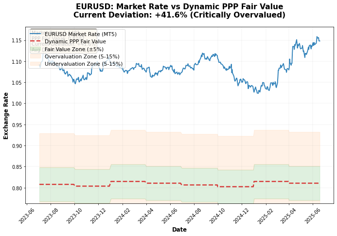
Running the system on data for 2024, I got some interesting results:

• EURUSD: fair rate 0.8753, market rate 1.0850 → EUR overvalued 
• GBPUSD: fair rate 0.8288, market rate 1.2650 → GBP overvalued 
• USDJPY: fair rate 136.20, market rate 148.50 → JPY undervalued
• USDCHF: fair rate 1.150, market rate 0.8850 → CHF overvalued

The most interesting result was for JPY. All four methods unanimously showed that at the rate of 148+ JPY is seriously undervalued. The confidence score comprised 0.85, one of the highest.

I did not create a separate trading system based on PPP. Instead, I integrated calculations with existing algorithms as an additional filter.

The logic is simple: if a technical system gives a signal to buy a currency that is significantly overvalued in terms of PPP, the position size is reduced or the signal is ignored. And vice versa, signals in the direction of PPP imbalance are strengthened.

Further plans for the system development

The current version of the system is just the beginning

I am planning several directions of development. Machine learning will help dynamically adjust the weights of methods based on historical accuracy and current conditions. Alternative data sources will include OECD data, cost of living indices, Big Mac real prices, satellite data and social sentiment. Expanding to include cryptocurrencies, commodities, stocks, and bonds will open up new opportunities. Automated trading with dynamic hedging and integration with brokerage APIs will make the system completely independent. Real-time monitoring with a web dashboard will complete the picture.

What I learned about PPP and foreign exchange markets?

A few months of work on this project gave me more knowledge about the currency markets than years of technical analysis. The PPP works, but not as I expected.

This is a compass for long-term direction, not a get-rich-quick magic formula. Deviations are corrected over months and years, not days and weeks. Data quality is critical — I spent more time searching and validating data than I spent on implementing the algorithms.

Simplicity beats complexity - five simple methods work better than any neural networks. PPP trading requires patience, which most traders lack. Fundamental analysis provides a link to economic reality in the era of algorithmic trading. A code is just a tool for solving a real problem.

Results and conclusions

The project began as a simple curiosity: is it possible to calculate fair exchange rates independently? It ended with the creation of a complete analysis system that helps make more informed trading decisions.

The journey from idea to working code took several months, hundreds of hours of studying economic theory, dozens of algorithm iterations, and countless hours of debugging. But the result was worth it.

The most important thing I realized is that there is no need to reinvent the wheel or chase complexity. Sometimes the best algorithm is a well-implemented classic. Purchasing power parity worked 500 years ago, it works now and will work in the future. We just need to use it correctly.

The complete source code of the system is available as an open source project. I welcome community contributions in the form of new data sources, alternative PPP calculation methods, error handling improvements, integration with brokerage APIs, and backtesting on historical data. If you are into Forex trading or quantitative analysis, give this system a try — it might just change the way you view the markets.