Mining Central Bank Balance Sheet Data to Get a Picture of Global Liquidity

The financial crises of the 21st century — from the mortgage meltdown of 2008 to the pandemic turmoil of the 2020s — have radically changed the rules of the game. Central banks are no longer limited to the modest role of interest rate regulators. Their arsenal has expanded to include exotic instruments: corporate bond purchases, direct bank lending, currency swaps, and even government spending financing. These measures, like powerful pumps, inject liquidity into — or withdraw it from — the global economy, and their effects are reflected in central bank balance sheets, the mirrors of monetary policy.

This article is not just a guide to analyzing central bank balance sheets. It is an in-depth exploration of how to build a system that, like an alchemical cauldron, transforms raw liquidity data into golden forecasts of currency pair movements. We will combine information from the US Federal Reserve (Fed), the European Central Bank (ECB), the Bank of Japan (BOJ) and the People's Bank of China (PBoC) to create a composite index of global liquidity. We will explore how machine learning and technical analysis can work in tandem to uncover hidden patterns traditional methods often fail to capture. Moreover, we will show how to integrate this system with real trading, turning abstract data into concrete trading decisions.

Traditional technical analysis, with its charts and indicators, often resembles attempts to predict the weather by looking only at the clouds. Fundamental analysis, on the other hand, requires a deep understanding of macroeconomics, which is not always suitable for quick trading decisions. Our approach bridges the gap between two worlds, where liquidity data becomes key to understanding both short-term movements and long-term trends. 

Theoretical foundations: Liquidity as the pulse of the global economy

Global liquidity is not simply the amount of money in circulation. It is the lifeblood of the global economy, a complex system that unites monetary aggregates, financial instruments and mechanisms that ensure the free flow of capital. In a narrow sense, liquidity is the ability of an asset to be quickly converted into money without losing value. But on a global scale, it reflects how easily capital moves between countries, markets and sectors. Capital flows themselves are capable of generating powerful long-term trends.

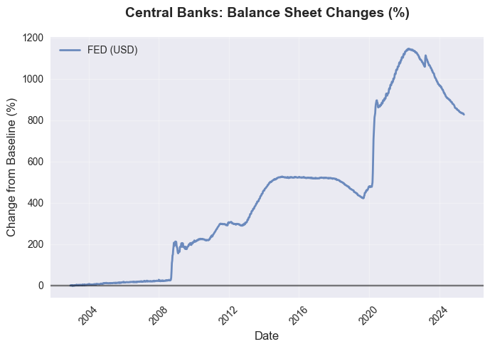
Central banks – the Fed, the ECB, the BOJ, the PBoC – are the main conductors of this orchestra. Their balance sheets are not just accounting reports, but indicators of how much money they have injected into the economy through asset purchases, lending, or other measures. When the Fed buys government bonds, it creates new liquidity by increasing its balance sheet. When the ECB raises reserve requirements, it withdraws liquidity, narrowing money flows.

Increasing the central bank's balance sheet through quantitative easing or asset purchases usually weakens the national currency. This happens for two reasons. Firstly, the growth of the money supply reduces the value of the currency according to the laws of supply and demand. Secondly, such measures are often accompanied by lower interest rates, making the currency less attractive to investors seeking yield.

However, this connection is not so simple. If all major central banks expand their balance sheets simultaneously, the effect on currency pairs may be minimal — all currencies "inflate" in sync. The key factor becomes relative momentum: if the BOJ expands its balance sheet faster than the Fed, JPY is likely to weaken against USD.

Understanding how liquidity is transmitted through the financial system is critical for forecasting. There are several channels:

• Interest-rate channel: Central bank rate cuts increase the money supply, which reduces the yield on currency-denominated assets and weakens the currency.
• Portfolio channel: Massive asset purchases by central banks alter the composition of investors’ portfolios, forcing them to seek alternative investments.
• Credit channel: Improving credit conditions stimulates economic activity and affects currency flows.
• Expectations channel: Communication and leading signals from central banks shape market expectations even before actual actions. 

Expectations for future policy  give birth to future trends. Let's now look at this in more detail.

In the era of information transparency, central banks have become masters of communication. Their statements, press conferences and forecasts are not just words, but powerful tools that shape market expectations. When the Fed chairman hints at tightening policy, markets may start selling USD even before the official decision. Liquidity analysis must take into account not only the numbers on balance sheets, but also the rhetoric of officials, which can be as important as their actual actions.

System architecture: Engineering the financial future

Our system is not a monolith, but a carefully constructed mosaic, where each module performs a clearly defined function. GlobalLiquidityMiner collects and processes data on central bank balance sheets, transforming chaotic information flows into coherent time series. ForexLiquidityForecaster uses this data, enriching it with technical indicators and running it through machine learning algorithms to create accurate forecasts. This approach allows updating individual components without disrupting the entire system, and adapting it to new data sources or market conditions.

Financial markets are complex adaptive systems where short-term trader sentiment is intertwined with long-term macroeconomic trends. Our architecture reflects this duality by combining fast technical signals with deep fundamental factors.

The GlobalLiquidityMiner module is the heart of the data collection system. It works with a variety of sources, from the Fed's FRED API to complex BOJ data formats and limited PBoC information. The main task is not just to load the data, but to standardize it for analysis. Different banks publish data at different frequencies (weekly Fed reports versus quarterly PBoC data) and in different currencies. The module interpolates missing values, normalizes indicators, and synchronizes time series.

import pandas as pd
import logging
from typing import Dict
from fredapi import Fred
import yfinance as yf
import requests
from io import StringIO

logger = logging.getLogger(__name__)

class GlobalLiquidityMiner:
    def __init__(self, fred_api_key: str, start_date: str, end_date: str):
        self.fred = Fred(api_key=fred_api_key) if fred_api_key else None
        self.start_date = start_date
        self.end_date = end_date
        self.data_cache = {}

    def fetch_central_bank_balance_sheets(self) -> Dict[str, pd.DataFrame]:
        """Obtaining central bank balance sheet data."""
        balance_sheets = {}
        
        if self.fred:
            logger.info("Loading Federal Reserve data...")
            try:
                fed_total_assets = self.fred.get_series('WALCL', start=self.start_date, end=self.end_date)
                fed_securities = self.fred.get_series('WSHOSHO', start=self.start_date, end=self.end_date)
                fed_loans = self.fred.get_series('WLRRAL', start=self.start_date, end=self.end_date)
                
                balance_sheets['FED'] = pd.DataFrame({
                    'date': fed_total_assets.index,
                    'total_assets': fed_total_assets.values,
                    'securities_held': fed_securities.reindex(fed_total_assets.index, method='ffill').values,
                    'loans_and_repos': fed_loans.reindex(fed_total_assets.index, method='ffill').values,
                    'currency': 'USD'
                })
                
                balance_sheets['FED']['assets_growth_rate'] = balance_sheets['FED']['total_assets'].pct_change(periods=52)
                balance_sheets['FED']['securities_share'] = balance_sheets['FED']['securities_held'] / balance_sheets['FED']['total_assets']
                
                logger.info(f"Loaded {len(fed_total_assets)} Federal Reserve data entries")
            except Exception as e:
                logger.error(f"Error loading Fed data: {e}")
        
        self.data_cache['balance_sheets'] = balance_sheets
        return balance_sheets

The module combines liquidity data with technical indicators, creating features for machine learning models. The use of sliding windows allows us to take into account the short-term and long-term effects of changes in liquidity.

from sklearn.ensemble import RandomForestRegressor
from sklearn.preprocessing import StandardScaler
from sklearn.metrics import r2_score, mean_squared_error
import numpy as np

class ForexLiquidityForecaster:
    def __init__(self, liquidity_miner: GlobalLiquidityMiner):
        self.liquidity_miner = liquidity_miner
        self.models = {}
        self.scalers = {}
        
    def build_prediction_model(self, symbol: str, feature_df: pd.DataFrame):
        """ Training a forecasting model."""
        targets = {
            f'return_{h}d': feature_df['close'].shift(-h) / feature_df['close'] - 1
            for h in [1, 5]
        }
        
        feature_columns = [col for col in feature_df.columns if not col.startswith(('return_', 'volatility_', 'direction_'))]
        X = feature_df[feature_columns].dropna()
        
        train_size = int(len(X) * 0.8)
        X_train, X_test = X.iloc[:train_size], X.iloc[train_size:]
        
        models = {}
        for target_name, target_series in targets.items():
            y = target_series.dropna()
            common_idx = X.index.intersection(y.index)
            X_aligned, y_aligned = X.loc[common_idx], y.loc[common_idx]
            
            scaler = StandardScaler()
            X_train_scaled = scaler.fit_transform(X_aligned.iloc[:train_size])
            X_test_scaled = scaler.transform(X_aligned.iloc[train_size:])
            
            model = RandomForestRegressor(n_estimators=100, max_depth=10, random_state=42)
            model.fit(X_train_scaled, y_aligned.iloc[:train_size])
            
            test_pred = model.predict(X_test_scaled)
            test_r2 = r2_score(y_aligned.iloc[train_size:], test_pred)
            
            models[target_name] = {'model': model, 'scaler': scaler, 'r2': test_r2}
        
        self.models[symbol] = models
        self.scalers[symbol] = scaler

The ForexLiquidityForecaster module is the brain of the system, where liquidity data meets market indicators. It uses Random Forest to identify non-linear relationships between central bank balance sheets, technical indicators (RSI, MACD, moving averages) and currency pair movements. Features are created taking into account time lags to capture both immediate and delayed effects of liquidity changes.

from sklearn.ensemble import RandomForestRegressor
from sklearn.preprocessing import StandardScaler
from sklearn.metrics import r2_score
import numpy as np
import pandas as pd

class ForexLiquidityForecaster:
    def __init__(self, liquidity_miner: GlobalLiquidityMiner):
        self.liquidity_miner = liquidity_miner
        self.models = {}
        self.scalers = {}
        self.forecasts = {}

    def prepare_features(self, symbol: str, historical_data: pd.DataFrame) -> pd.DataFrame:
        """Create features for forecasting."""
        df = historical_data.copy()
        
        # Technical indicators
        df['rsi_14'] = self.calculate_rsi(df['close'], 14)
        df['ema_50'] = df['close'].ewm(span=50).mean()
        df['volatility_20d'] = df['close'].pct_change().rolling(20).std()
        
        # Attaching liquidity data
        if 'balance_sheets' in self.liquidity_miner.data_cache:
            for bank, bs_data in self.liquidity_miner.data_cache['balance_sheets'].items():
                df = df.join(bs_data[['total_assets']].rename(columns={'total_assets': f'{bank}_balance'}), how='left')
                df[f'{bank}_balance'].fillna(method='ffill', inplace=True)
        
        return df.dropna()

    def calculate_rsi(self, series: pd.Series, period: int = 14) -> pd.Series:
        """RSI calculation."""
        delta = series.diff()
        gain = delta.where(delta > 0, 0).rolling(window=period).mean()
        loss = -delta.where(delta < 0, 0).rolling(window=period).mean()
        rs = gain / loss
        return 100 - (100 / (1 + rs))

    def build_prediction_model(self, symbol: str, feature_df: pd.DataFrame):
        """ Training a forecasting model."""
        targets = {
            f'return_{h}d': feature_df['close'].shift(-h) / feature_df['close'] - 1
            for h in [1, 3, 5, 8]
        }
        
        feature_columns = [col for col in feature_df.columns if not col.startswith('return_')]
        X = feature_df[feature_columns].dropna()
        
        train_size = int(len(X) * 0.8)
        X_train, X_test = X.iloc[:train_size], X.iloc[train_size:]
        
        models = {}
        for target_name, target_series in targets.items():
            y = target_series.dropna()
            common_idx = X.index.intersection(y.index)
            X_aligned, y_aligned = X.loc[common_idx], y.loc[common_idx]
            
            scaler = StandardScaler()
            X_train_scaled = scaler.fit_transform(X_aligned.iloc[:train_size])
            X_test_scaled = scaler.transform(X_aligned.iloc[train_size:])
            
            model = RandomForestRegressor(n_estimators=200, max_depth=15, random_state=42)
            model.fit(X_train_scaled, y_aligned.iloc[:train_size])
            
            test_pred = model.predict(X_test_scaled)
            test_r2 = r2_score(y_aligned.iloc[train_size:], test_pred)
            
            models[target_name] = {'model': model, 'scaler': scaler, 'r2': test_r2}
        
        self.models[symbol] = models
        self.scalers[symbol] = scaler

Practical implementation: From data to action

The FRED API is a treasure trove of data on the Federal Reserve's balance sheet, including total assets, securities, and loans. The code handles API limitations such as request limits and synchronizes data at different intervals.

def fetch_fed_data(self):
    """Obtaining Federal Reserve data via API FRED."""
    try:
        fed_data = self.fred.get_series('WALCL', start=self.start_date, end=self.end_date)
        return pd.DataFrame({
            'date': fed_data.index,
            'total_assets': fed_data.values,
            'currency': 'USD'
        }).set_index('date')
    except Exception as e:
        logger.error(f"Error loading Fed data: {e}")
        return pd.DataFrame()

For the ECB, data is retrieved via the Statistical Data Warehouse, and in case of outages, proxy indicators, such as EURUSD and Euro Stoxx 50, are used. For BOJ and PBoC, where data access is limited, market indicators (Nikkei 225, USDJPY, Chinese bonds) are used.

def fetch_boj_proxy_data(self):
    """Obtaining BOJ proxy data."""
    try:
        usdjpy = yf.download('USDJPY=X', start=self.start_date, end=self.end_date, progress=False)
        nikkei = yf.download('^N225', start=self.start_date, end=self.end_date, progress=False)
        
        proxy_balance = pd.DataFrame(index=usdjpy.index)
        proxy_balance['jpy_strength'] = 1 / usdjpy['Close']
        proxy_balance['equity_liquidity'] = nikkei['Close'] / nikkei['Close'].rolling(252).mean()
        proxy_balance['synthetic_balance'] = proxy_balance['jpy_strength'].rolling(30).mean() * proxy_balance['equity_liquidity'] * 1000000
        
        return proxy_balance
    except Exception as e:
        logger.error(f"Error loading BOJ data: {e}")
        return pd.DataFrame()

Liquidity index: Creating a financial compass

The Composite Liquidity Index combines normalized data from central bank balance sheets with weights reflecting their influence: Fed (35%), ECB (25%), BOJ (15%), PBoC (20%), others (5%). Dynamic adjustment takes into account data volatility and reliability.

def calculate_liquidity_index(self) -> pd.DataFrame:
    """Calculation of the composite liquidity index."""
    all_series = {}
    weights = {'FED_balance': 0.35, 'ECB_balance': 0.25, 'BOJ_balance': 0.15, 'PBOC_balance': 0.20}
    
    for bank, df in self.data_cache.get('balance_sheets', {}).items():
        series_name = f'{bank}_balance'
        normalized = (df['total_assets'] - df['total_assets'].rolling(252).mean()) / df['total_assets'].rolling(252).std()
        all_series[series_name] = normalized
    
    combined_df = pd.DataFrame(all_series).fillna(method='ffill')
    liquidity_index = combined_df.dot(pd.Series(weights))
    
    return pd.DataFrame({'liquidity_index': liquidity_index}, index=combined_df.index)

In addition to the main index, the system creates sub-indices: short-term (30 days), long-term (252 days), acceleration index and liquidity volatility index. These indicators help adapt forecasts to different market conditions.

def enhance_liquidity_index(self, base_index: pd.Series) -> pd.DataFrame:
    """Creating advanced liquidity indicators."""
    enhanced_df = pd.DataFrame(index=base_index.index)
    enhanced_df['base_liquidity_index'] = base_index
    enhanced_df['short_term_liquidity'] = base_index.rolling(window=30).mean()
    enhanced_df['long_term_trend'] = base_index.rolling(window=252).mean()
    enhanced_df['liquidity_acceleration'] = base_index.diff().diff()
    enhanced_df['liquidity_volatility'] = base_index.rolling(window=60).std()
    
    return enhanced_df

Integration with MetaTrader 5: A bridge to real trading

The system integrates with MetaTrader 5 to retrieve market data and generate trading signals. The features include both technical indicators and liquidity metrics, creating a unique data set for forecasting.

import MetaTrader5 as mt5
from datetime import datetime, timedelta

class TradingIntegration:
    def __init__(self, forecaster: ForexLiquidityForecaster):
        self.forecaster = forecaster
        mt5.initialize()
    
    def fetch_forex_data(self, symbol: str, days: int = 1460) -> pd.DataFrame:
        """Fetching data from MetaTrader 5."""
        utc_from = datetime.now() - timedelta(days=days)
        rates = mt5.copy_rates_from(symbol, mt5.TIMEFRAME_D1, utc_from, days)
        
        if rates is None:
            return pd.DataFrame()
        
        df = pd.DataFrame(rates)
        df['date'] = pd.to_datetime(df['time'], unit='s')
        df.set_index('date', inplace=True)
        return df
    
    def generate_trading_signals(self, symbol: str, forecasts: dict) -> dict:
        """Generating trading signals."""
        signals = {}
        short_term_returns = [f['return'] for h, f in forecasts['forecasts'].items() if h in ['1d', '2d', '3d']]
        avg_return = np.mean(short_term_returns) if short_term_returns else 0
        
        signals['short_term'] = {
            'signal': 'BUY' if avg_return > 0.005 else 'SELL' if avg_return < -0.005 else 'HOLD',
            'strength': min(abs(avg_return) * 100, 100)
        }
        
        return signals

Visualization: A picture of the world in graphs

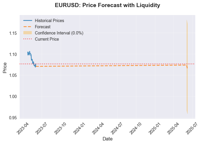
The system creates interactive visualizations that help traders see the relationship between liquidity and prices. The charts include price forecasts, liquidity index dynamics and feature importance.

import matplotlib.pyplot as plt
import numpy as np

def create_comprehensive_visualization(self, symbol: str):
    """Building a set of visualizations."""
    forecasts = self.forecaster.forecasts.get(symbol, {})
    historical_data = self.fetch_forex_data(symbol, days=180)
    
    plt.figure(figsize=(15, 8))
    plt.plot(historical_data.index[-60:], historical_data['close'].iloc[-60:], label='Historical prices', linewidth=2)
    
    forecast_dates = [datetime.strptime(f['date'], '%Y-%m-%d') for f in forecasts.get('forecasts', {}).values()]
    forecast_prices = [f['price'] for f in forecasts.get('forecasts', {}).values()]
    
    if forecast_dates:
        plt.plot(forecast_dates, forecast_prices, 'r--', label='Forecast', linewidth=2)
    
    plt.title(f'{symbol}: Price forecast considering liquidity', fontsize=14, fontweight='bold')
    plt.xlabel('Date', fontsize=12)
    plt.ylabel('Price', fontsize=12)
    plt.legend()
    plt.grid(True, alpha=0.3)
    plt.savefig(f'forecast_{symbol}.png', dpi=300)
    plt.close()

As a result, we obtain a picture of global liquidity:

Forecasts derived from it:

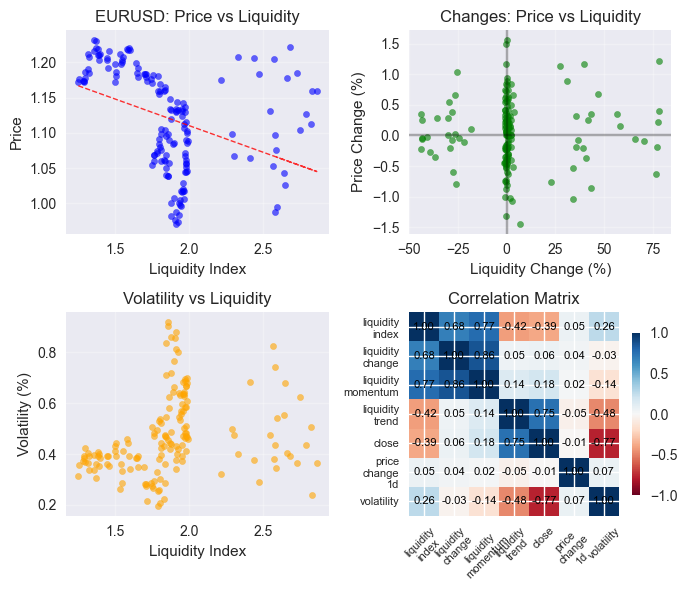
And the correlation matrix:

Conclusion

The developed system is a powerful tool that combines central bank balance sheet analysis with advanced machine learning and technical analysis techniques, providing a comprehensive approach to forecasting currency movements. Modular system architecture including GlobalLiquidityMiner and ForexLiquidityForecaster provides flexibility, scalability and the ability to adapt to changing market conditions.

Integration with MetaTrader 5 allows traders to apply forecasts to real trading, turning complex data into concrete trading decisions. Interactive visualizations and backtest results enhance the transparency and robustness of the system, empowering traders to make informed decisions with a high degree of confidence.

This system goes beyond traditional analysis, offering a holistic approach that takes into account both fundamental and technical factors. It allows traders to not only react to market changes, but also anticipate them, using global liquidity as a compass in the stormy seas of the forex market. In the face of increasing volatility and uncertainty in the global economy, this approach is becoming not just an advantage, but a necessity for successful trading.

The system is not without limitations. Limited access to data from some central banks, such as the PBoC, requires the use of proxy indicators, which may reduce accuracy. Furthermore, machine learning, despite its power, does not guarantee absolute forecast accuracy, especially in the face of unexpected geopolitical or economic shocks. However, continuous improvement of algorithms, expansion of data sources, and consideration of new market factors will allow the system to remain relevant and effective.

Future development of the system may include integration with neural network models to process large volumes of unstructured data, such as news and social media, which will enhance its predictive power. It is also possible to implement adaptive mechanisms that automatically adjust the liquidity index weights depending on current economic conditions. This paves the way for the creation of a new generation of trading systems that will be even more resilient to uncertainty and capable of delivering stable results in any market conditions.