Neural Networks in Trading: Adaptive Detection of Market Anomalies (DADA)

Introduction

With the advancement of technology and the automation of processes, time series have become an integral part of financial market analysis. Effective detection of anomalies in market data makes it possible to promptly identify potential threats such as sharp price fluctuations, asset manipulation, and changes in liquidity. This is especially important for algorithmic trading, risk management, and the assessment of financial system stability. Sudden spikes in volatility, deviations in trading volumes, or unusual correlations between assets may signal failures, speculative activity, or even market crises.

Modern anomaly detection methods based on deep learning have achieved significant success, but they have limitations. Most often, such approaches require separate training for each new dataset, which hinders their application in real-world conditions. Financial data is constantly changing, and its historical patterns do not always repeat.

One of the main problems is the varying structure of data across different markets. Modern algorithms typically use autoencoders to "memorize" normal market behavior, since anomalies occur rarely. However, if a model retains too much information, it begins to account for market noise, reducing anomaly detection accuracy. Conversely, excessive compression may lead to the loss of important patterns. Most approaches use a fixed compression ratio, which limits the model's ability to adapt to different market conditions.

Another challenge is the diversity of anomalies. Many models are trained only on normal data, but without understanding anomalies themselves, they are difficult to detect. For example, a sharp price spike may be an anomaly in one market but a normal occurrence in another. In some assets, anomalies are associated with sudden liquidity surges, while in others - with unexpected correlations. As a result, a model may either miss important signals or generate too many false signals.

To address these issues, the authors of "Towards a General Time Series Anomaly Detector with Adaptive Bottlenecks and Dual Adversarial Decoders" proposed a new framework DADA which uses adaptive information compression and two independent decoders. Unlike traditional methods, DADA flexibly adapts to different data. Instead of a fixed compression level, it employs multiple options and selects the most suitable one for each case. This helps better capture the characteristics of market data and preserve important patterns.

At the model output, two decoders are used. One decoder is used for normal data, while the other handels anomalous data. The first decoder learns to reconstruct the time series, while the second is trained on anomalous examples. This enables clear separation between normal behavior and anomalies, while also reducing the likelihood of false signals.

The DADA Algorithm

Time series are sequences of data that change over time. Any deviations from normal data behavior may signal crises, failures, or fraudulent activity. To effectively identify such anomalies, the DADA framework (Detector with Adaptive Bottlenecks and Dual Adversarial Decoders) employs deep learning methods for adaptive time series analysis and anomaly pattern detection. A key feature of DADA is its universality. It does not require prior adaptation to a specific domain and can operate on a wide range of input data.

The DADA framework is based on the idea of data reconstruction using masking, which makes it an effective tool for analyzing temporal dependencies and identifying deviations from the norm. This method allows the model not just to memorize patterns in the data, but to learn to understand their structure by reconstructing missing or corrupted segments.

The training process involves working with two types of sequences: normal and anomalous. Unlike traditional approaches that require manual labeling of anomalous data, the authors of the DADA framework used a generative approach, adding artificial noise to the original time series. This approach not only simplifies data preparation by eliminating manual labor, but also makes the model more universal. It learns to detect various types of deviations: spikes, outliers, trend shifts, changes in volatility, and other patterns.

At the first stage, the original data is divided into segments (patches), to which random masking is applied. This is necessary for training the model to reconstruct missing parts of the data. It enhances its ability to detect anomalies and hidden patterns.

Next, the segments are fed into an encoder, where they are transformed into a compact latent representation. The encoder learns to extract key features of the time series while ignoring noise and insignificant details. This approach allows the model to generalize better and work with data of different nature, whether price charts in financial markets, trading volume time series, or other indicators.

One of the key components of the model is the adaptive bottleneck mechanism, which regulates the degree of information compression depending on the structure and quality of the data. When the data contains a meaningful signal, the model retains more detail; when the information is redundant or heavily noisy, compression is increased, helping to minimize interference and improve anomaly detection.

The Adaptive Bottleneck Module (AdaBN) dynamically adjusts the degree of data compression. This mechanism consists of a pool of small models resembling autoencoders. Each of them has a latent representation of a different size:

where DownNeti(•) performs compression of the analyzed data, UpNeti(•) reconstructs it.

An adaptive router selects the optimal path based on analysis of the input data:

where Wrouter and Wnoise are trainable matrices.

For compressing each segment, the k most suitable routes with the highest value of R(z) are used.

After encoding, the latent representations are passed to two parallel decoders. One of them is designed to reconstruct normal data and is trained to minimize reconstruction error. The second is intended to detect anomalies by creating maximum divergence between reconstructed and original values. This adversarial process allows the model to effectively distinguish between standard patterns and unexpected deviations.

During testing and real-world deployment, the anomalous decoder is disabled, and evaluation is performed exclusively using the normal decoder. If the model reconstructs the data with high accuracy, the time series corresponds to normal behavior. If reconstruction is accompanied by significant errors, this indicates a potential anomaly.

The authors' visualization of the DADA framework is presented below.

Implementation Using MQL5

After reviewing the theoretical aspects of the DADA framework, we move on to the practical part of our work, where we consider an implementation of our own interpretation of the proposed approaches in MQL5. The key element of this framework is the adaptive bottleneck module. We begin our work with its construction.

I believe I am not the only one who noticed its similarity to the previously implemented Mixture of Experts module. However, there is one important difference. In the CNeuronMoE object we constructed, the use of mini-models with identical architecture is assumed. In this case, however, we need to vary the size of the latent state layer for each model, adapting them to different data characteristics. This option can no longer be implemented using convolutional layer objects as was done previously. Of course, each model could be created separately and the data passed through them sequentially. However, this leads to reduced hardware efficiency and increased costs for training and deployment.

To eliminate these issues, it was decided to develop a new object for a multi-window convolutional layer. It is based on the idea of simultaneously using several variants of convolution window sizes. This allows the model to analyze data at different levels of granularity in parallel computational streams. Such an approach makes the architecture more flexible, improves the quality of input data processing, and enables more efficient use of computational resources. As a result, the model can better adapt to various temporal structures in the input data, ensuring high accuracy and performance.

Constructing Algorithms on the OpenCL Program Side

As usual, the bulk of mathematical operations is transferred into the OpenCL context. Here, we create the FeedForwardMultWinConv kernel, within which we organize the forward pass of our new layer.

__kernel void FeedForwardMultWinConv(__global const float *matrix_w,
                                     __global const float *matrix_i,
                                     __global float *matrix_o,
                                     __global const int *windows_in,
                                     const int inputs,
                                     const int windows_total,
                                     const int window_out,
                                     const int activation
                                    )
  {
   const size_t i = get_global_id(0);
   const size_t v = get_global_id(1);
   const size_t outputs = get_global_size(0);

The kernel parameters include pointers to four data buffers and four constants that define the structure of the input data and the results.

Note that one of the global buffers (windows_in) contains integer values. It stores the sizes of the convolution windows. It is assumed that the input data buffer (matrix_i) contains a sequence of segments. Within each segment, the data for each convolution window is arranged sequentially.

We plan to invoke this kernel in a two-dimensional task space. The size of the first dimension indicates the number of values in the result buffer for each univariate sequence, while the second dimension represents the number of such univariate sequences.

It should be clarified that the first dimension refers specifically to the number of values in the result buffer, not the number of elements in the univariate sequence. In other words, the size of the first dimension equals the product of the number of analyzed segments in the univariate sequence and the number of filters and convolution windows used. At the same time, each element uses the same number of filters regardless of the convolution window size. This is necessary to ensure consistency in the formats of data reconstructed from the compressed representation.

Inside the kernel body, we first identify the current thread in the two-dimensional task space for each dimension.

Next, it is necessary to determine offsets in the global data buffers to access the required elements. Clearly, the thread identifier in the first dimension points to an element of the result buffer within the analyzed univariate sequence. However, determining offsets in the remaining data buffers requires additional work.

First, we determine the position of the element within the analyzed segment. To do this, we take the remainder of the division of the first-dimension thread identifier by the total number of elements in the result buffer for a single segment.

   const int id = i % (window_out * windows_total);

We then prepare several local variables to temporarily store intermediate values.

   int step = 0;
   int shift_in = 0;
   int shift_weight = 0;
   int window_in = 0;
   int window = 0;

Next, we organize a loop to iterate over all values in the convolution window buffer.

#pragma unroll
   for(int w = 0; w < windows_total; w++)
     {
      int win = windows_in[w];
      step += win;

Within the loop, we compute the sum of all convolution windows, which gives us the size of a single segment in the input data buffer. Additionally, within this loop, we determine the offset within the current segment to the required convolution window (shift_in), the size of the analyzed convolution window (window_in), and the offset in the trainable parameter buffer to the beginning of the matrix elements of the required convolution window (shift_weight).

      if((w * window_out) < id)
        {
         shift_in = step;
         window_in = win;
         shift_weight += (win + 1) * window_out;
        }
     }

Next, we determine the number of complete segments preceding the current element in the result buffer (steps) and add the corresponding offset in the input data buffer to reach the required segment.

   int steps = (int)(i / (window_out * windows_total));
   shift_in += steps * step + v * inputs;

To the offset in the trainable parameter buffer, we add a correction for the appropriate filter. To do this, we take the remainder of the division of the position of the analyzed element within the current segment of the result buffer. This gives us the index of the element within the results of the current convolution window. In essence, this value identifies the required filter. The number of trainable parameters in each filter equals the size of the convolution window plus the bias element. Thus, by multiplying the filter index by the number of trainable parameters, we obtain the required offset.   

shift_weight += (id % window_out) * (window_in+1);

After completing the preparatory steps, we organize a loop to compute the value of the current element into a local variable.

   float sum = matrix_w[shift_weight + window_in];
#pragma unroll
   for(int w = 0; w < window_in; w++)
      if((shift_in + w) < inputs)
         sum += IsNaNOrInf(matrix_i[shift_in + w], 0) * matrix_w[shift_weight + w];

The obtained value is then adjusted using the activation function and stored in the corresponding element of the global result buffer.

 matrix_o[v * outputs + i] = Activation(sum, activation);
}

After constructing the forward pass algorithm, we proceed to organize the backpropagation processes. Here, we first create the CalcHiddenGradientMultWinConv kernel to distribute error gradients down to the level of the input data. The structure of this kernel’s parameters largely follows that of the forward pass kernel. We only add pointers to the corresponding gradient buffers.

__kernel void CalcHiddenGradientMultWinConv(__global const float *matrix_w,
                                            __global const float *matrix_i,
                                            __global float *matrix_ig,
                                            __global const float *matrix_og,
                                            __global const int *windows_in,
                                            const int outputs,
                                            const int windows_total,
                                            const int window_out,
                                            const int activation
                                           )
  {
   const size_t i = get_global_id(0);
   const size_t v = get_global_id(1);
   const size_t inputs = get_global_size(0);

This kernel also operates in a two-dimensional task space. However, this time the first dimension indicates the offset in the input data buffer, since it is at the input data level that we need to aggregate gradient values from all filters.

As usual, the kernel first identifies the thread across all dimensions of the task space. Then, we organize a loop to sum all convolution windows in order to determine the size of a single segment in the input data buffer.

   int step = 0;
#pragma unroll
   for(int w = 0; w < windows_total; w++)
      step += windows_in[w];

This allows us to determine the index of the segment corresponding to the analyzed element and the offset within that segment.

int steps = (int)(i / step);
int id = i % step;

Next, we declare several local variables for temporary data storage and organize another loop. Within this loop, we determine the size of the analyzed convolution window (window_in), the index of the convolution window (window), and the offset within the current segment to the beginning of the current convolution window (before).

   int window = 0;
   int before = 0;
   int window_in = 0;
#pragma unroll
   for(int w = 0; w < windows_total; w++)
     {
      window_in = windows_in[w];
      if((before + window_in) >= id)
         break;
      window = w + 1;
      before += window_in;
     }

These values allow us to determine the offset in the result buffer (shift_out) and in the parameter tensor (shift_weight).

int shift_weight = (before + window) * window_out + id - before;
int shift_out = (steps * windows_total + window) * window_out + v * outputs;

At this point, the preparatory phase is complete, and we have sufficient information to accumulate the error gradients. We organize another loop in which we collect gradient values from all filters, taking into account the corresponding weights.

   float sum = 0;
#pragma unroll
   for(int w = 0; w < window_out; w++)
      sum += IsNaNOrInf(matrix_og[shift_out + w], 0) * matrix_w[shift_weight + w * (window_in + 1)];

The resulting value is adjusted using the derivative of the activation function of the input layer, and the result is stored in the corresponding element of the global gradient buffer.

 matrix_ig[v * inputs + i] = Deactivation(sum, matrix_i[v * inputs + i], activation);
}

The third stage of our work is to construct the process of distributing the error gradient to the level of the weight coefficients and updating them to minimize the overall model error. Within this work, we implement the Adam optimization algorithm in the UpdateWeightsMultWinConvAdam kernel.

To correctly construct this algorithm, we expand the number of kernel parameters by adding specific constants and two global buffers for the moments.

__kernel void UpdateWeightsMultWinConvAdam(__global float *matrix_w,
                                           __global const float *matrix_og,
                                           __global const float *matrix_i,
                                           __global float *matrix_m,
                                           __global float *matrix_v,
                                           __global const int *windows_in,
                                           const int windows_total,
                                           const int window_out,
                                           const int inputs,
                                           const int outputs,
                                           const float l,
                                           const float b1,
                                           const float b2
                                          )
  {
   const size_t i = get_global_id(0);  // weight shift
   const size_t v = get_local_id(1);   // variable
   const size_t variables = get_local_size(1);

This kernel is also intended to be used in a two-dimensional task space. This time, the first dimension indicates the optimized element in the global buffer of trainable parameters. However, there is an important nuance. When working with multidimensional time series, each univariate sequence is analyzed using shared trainable parameters. Therefore, at this stage, we need to aggregate error gradients from all univariate sequences. To organize parallel processing of individual univariate sequences, we distribute them along the second dimension of the task space, while grouping them into workgroups to enable data exchange. It is precisely for data exchange within a workgroup that we create an array in the local memory of the OpenCL context.

__local float temp[LOCAL_ARRAY_SIZE];

Next, we proceed to the preparatory stage, where we determine offsets in the data buffers. Perhaps the simplest step is determining the stride in the result buffer (step_out). It is equal to the product of the number of convolution windows per segment and the number of filters.

int step_out = window_out * windows_total;

To obtain the remaining parameters, additional work is required. First, we declare local variables to store intermediate results.

int step_in = 0;
int shift_in = 0;
int shift_out = 0;
int window = 0;
int number_w = 0;

Then, we organize a loop to iterate over the values in the global buffer of convolution window sizes.

#pragma unroll
   for(int w = 0; w < windows_total; w++)
     {
      int win = windows_in[w];
      if((step_in + w)*window_out <= i &&
         (step_in + win + w + 1)*window_out > i)
        {
         shift_in = step_in;
         shift_out = (step_in + w + 1) * window_out;
         window = win;
         number_w = w;
        }
      step_in += win;
     }

Within this loop, we determine the offset to the required convolution window in the input data buffers (shift_in) and result buffers (shift_out), the size of the convolution window (window), and its index in the buffer (number_w). In addition, we compute the sum of all convolution windows (step_in), which indicates the segment size. This value is also used as the stride for the input data buffer.

It is important to note that not every trainable parameter is associated with the input data buffer, due to the presence of the bias element. We therefore introduce a flag to detect such elements.

bool bias = ((i - (shift_in + number_w) * window_out) % (window + 1) == window);

Next, we adjust the offset to the required element in the result buffer.

int t = (i - (shift_in + number_w) * window_out) / (window + 1);
shift_out += t + v * outputs;

A similar operation is performed to adjust the offset in the global input data buffer.

   shift_in += (i - (shift_in + number_w) * window_out) % (window + 1) + v * inputs;

At this point, the preparatory phase is complete, and we proceed directly to determining the gradient of the analyzed parameter. To do this, we organize a loop that collects gradient values from all elements of the result buffer whose computation involved the parameter being optimized in the current thread.

   float grad = 0;
   int total = (inputs + step_in - 1) / step_in;
#pragma unroll
   for(int t = 0; t < total; t++)
     {
      int sh_out = t * step_out + shift_out;
      if(bias && sh_out < outputs)
        {
         grad += IsNaNOrInf(matrix_og[sh_out], 0);
         continue;
        }

For bias elements, we simply sum the gradient values, while for other parameters, we adjust them based on the corresponding element of the input data.

 int sh_in = t * step_in + shift_in;
 if(sh_in >= inputs)
    break;
 grad += IsNaNOrInf(matrix_og[sh_out] * matrix_i[sh_in], 0);
}

It should be noted that within this loop, we collect error values only within a single univariate sequence. However, as mentioned earlier, the optimized parameter is used across all sequences of the multidimensional time series. Therefore, before performing parameter optimization, we must aggregate values from all univariate sequences computed within the workgroup. To achieve this, at the first stage we sum individual values into elements of a local array.

//--- sum
   const uint ls = min((uint)variables, (uint)LOCAL_ARRAY_SIZE);
#pragma unroll
   for(int s = 0; s < (int)variables; s += ls)
     {
      if(v >= s && v < (s + ls))
         temp[v % ls] = (i == 0 ? 0 : temp[v % ls]) + grad;
      barrier(CLK_LOCAL_MEM_FENCE);
     }

Then, we sum the values accumulated in the elements of the local array.

   uint count = ls;
#pragma unroll
   do
     {
      count = (count + 1) / 2;
      if(v < ls)
         temp[v] += (v < count && (v + count) < ls ? temp[v + count] : 0);
      if(v + count < ls)
         temp[v + count] = 0;
      barrier(CLK_LOCAL_MEM_FENCE);
     }
   while(count > 1);

After obtaining the total error gradient from all threads in the workgroup, we can update the value of the analyzed parameter. Only a single thread is required for this operation.

   if(v == 0)
     {
      grad = temp[0];
      float mt = IsNaNOrInf(clamp(b1 * matrix_m[i] + (1 - b1) * grad, -1.0e5f, 1.0e5f), 0);
      float vt = IsNaNOrInf(clamp(b2 * matrix_v[i] + (1 - b2) * pow(grad, 2), 1.0e-6f, 1.0e6f), 1.0e-6f);
      float weight = clamp(matrix_w[i] + IsNaNOrInf(l * mt / sqrt(vt), 0), -MAX_WEIGHT, MAX_WEIGHT);
      matrix_w[i] = weight;
      matrix_m[i] = mt;
      matrix_v[i] = vt;
     }
  }

As a result of these operations, we update the value of the analyzed parameter and the corresponding moments in the global data buffers.

At this point, we complete the construction of the multi-window convolutional layer algorithms in our OpenCL program. The full source code is provided in the appendix.

Multi-Window Convolutional Layer Object

The next stage of our work is to integrate the previously constructed algorithms of the multi-window convolutional layer into the main program. For this purpose, we create a new object CNeuronMultiWindowsConvOCL, in which we organize the processes for managing the kernels created within the OpenCL context. The structure of the new object is presented below.

class CNeuronMultiWindowsConvOCL    :  public CNeuronConvOCL
  {
protected:
   int               aiWindows[];
   //---
   virtual bool      feedForward(CNeuronBaseOCL *NeuronOCL);
   virtual bool      updateInputWeights(CNeuronBaseOCL *NeuronOCL);
   virtual bool      calcInputGradients(CNeuronBaseOCL *NeuronOCL);

public:
                     CNeuronMultiWindowsConvOCL(void) {  activation = SoftPlus;  iWindow = -1; }
                    ~CNeuronMultiWindowsConvOCL(void) {};
   virtual bool      Init(uint numOutputs, uint myIndex, COpenCLMy *open_cl,
                          uint &windows[], uint window_out, uint units_count, uint variables,
                          ENUM_OPTIMIZATION optimization_type, uint batch);
   //---
   virtual int       Type(void)   const   {  return defNeuronMultiWindowsConvOCL;   }
   //--- methods for working with files
   virtual bool      Save(int const file_handle);
   virtual bool      Load(int const file_handle);
   //---
   virtual void      SetOpenCL(COpenCLMy *obj);
  };

Essentially, the new CNeuronMultiWindowsConvOCL object represents a modified version of a standard convolutional layer. Therefore, it is logical to derive it from the parent class. This allows us to inherit the basic convolution logic and avoid code duplication.

In the presented structure, we observe the familiar set of overridden virtual methods. However, the main difference of the new object lies in its simultaneous operation with multiple convolution window sizes. This requires the creation of additional data storage elements and interfaces for transferring them to the OpenCL context. To achieve this, we declare an additional array aiWindows and modify the parameters of the object initialization method Init.

bool CNeuronMultiWindowsConvOCL::Init(uint numOutputs, uint myIndex, COpenCLMy *open_cl,
                                      uint &windows[], uint window_out, uint units_count,
                                      uint variables, ENUM_OPTIMIZATION optimization_type, uint batch)
  {
   if(windows.Size() <= 0 || ArrayCopy(aiWindows, windows) < int(windows.Size()))
      return false;

It is important to emphasize that, despite all the changes introduced into the CNeuronMultiWindowsConvOCL algorithm, we have made every effort to preserve the logic and capabilities of the parent class. This not only simplifies integration of the new object into the existing architecture, but also allows reuse of already tested and debugged mechanisms.

The initialization algorithm of the object begins by checking the size of the convolution window array received in the parameters and copying its values into a specially created internal array.

Next, we determine the sum of all convolution windows, adding a bias element to each.

int window = 0;
for(uint i = 0; i < aiWindows.Size(); i++)
   window += aiWindows[i] + 1;

This may seem like a non-obvious but necessary operation. The reason is that for each convolution window we need to generate a weight matrix of size (Windowi + 1) * Filters. Thus, the total size of the parameter buffer will be:

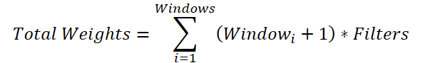
The common variable for the number of filters can be factored out of the summation:

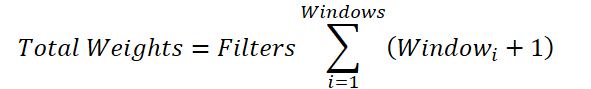
If we replace the sum of the windows with a total value, we arrive at the formula for determining the number of trainable parameters for a single convolution window. However, in the parent class, only one bias element can be added, rather than one per convolution window as required here. Therefore, we add a bias element for each window to the total sum, then decrement the resulting value by one and pass it as the window size and convolution stride to the parent class initialization method.

window--;
if(!CNeuronConvOCL::Init(numOutputs, myIndex, open_cl, window, window, window_out,
                         units_count * aiWindows.Size()*variables, 1, ADAM, batch))
   return false;

Since we plan to use identical parameters for all univariate sequences, we set their number to 1. At the same time, we increase the number of elements in the sequence by multiplying it by the number of convolution windows and univariate sequences.

This approach allows us to initialize all inherited data buffers with the required sizes, including initializing the buffer of trainable parameters with random values.

Next, we create a global data buffer to transfer the array of convolution windows into the OpenCL context. As expected, the values of this buffer are set during object initialization and remain unchanged during training and model operation. Therefore, the buffer is created only within the OpenCL context, while our object stores only a pointer to it.

   iVariables = variables;
   iWindow = OpenCL.AddBufferFromArray(aiWindows, 0, aiWindows.Size(), CL_MEM_READ_ONLY);
   if(iWindow < 0)
      return false;
//---
   return true;
  }

We verify the correctness of the global buffer creation using the returned handle and complete the initialization method of the new object, returning a boolean result of the operation to the calling program.

After initializing the new object, we proceed to override the feed-forward pass method CNeuronMultiWindowsConvOCL::feedForward. As you may have already guessed, this is where the previously created FeedForwardMultWinConv kernel is enqueued for execution. However, despite using a standard procedure for such cases, there are several nuances worth noting.

bool CNeuronMultiWindowsConvOCL::feedForward(CNeuronBaseOCL *NeuronOCL)
  {
   if(!OpenCL || !NeuronOCL)
      return false;

The method parameters include a pointer to the input data object, whose validity is immediately checked.

After successfully passing the validation checks, we initialize the task space arrays.

uint global_work_offset[2] = {0, 0};
uint global_work_size[2] = {Neurons() / iVariables, iVariables};

As mentioned earlier in the kernel description, the second dimension corresponds to the number of univariate sequences in the input data. The number of threads in the first dimension is determined by dividing the total number of elements in the result buffer of our object by the number of univariate sequences.

Next, the data is passed to the kernel parameters.

   ResetLastError();
   int kernel = def_k_FeedForwardMultWinConv;
   if(!OpenCL.SetArgumentBuffer(kernel, def_k_ffmwc_matrix_i, NeuronOCL.getOutputIndex()))
     {
      printf("Error of set parameter kernel %s: %d; line %d", __FUNCTION__, GetLastError(), __LINE__);
      return false;
     }
   if(!OpenCL.SetArgumentBuffer(kernel, def_k_ffmwc_matrix_o, getOutputIndex()))
     {
      printf("Error of set parameter kernel %s: %d; line %d", __FUNCTION__, GetLastError(), __LINE__);
      return false;
     }
   if(!OpenCL.SetArgumentBuffer(kernel, def_k_ffmwc_matrix_w, WeightsConv.GetIndex()))
     {
      printf("Error of set parameter kernel %s: %d; line %d", __FUNCTION__, GetLastError(), __LINE__);
      return false;
     }
   if(!OpenCL.SetArgumentBuffer(kernel, def_k_ffmwc_windows_in, iWindow))
     {
      printf("Error of set parameter kernel %s: %d; line %d", __FUNCTION__, GetLastError(), __LINE__);
      return false;
     }

It is worth noting that the previously stored handle is passed as the convolution window size buffer. Meanwhile, the dimensionality of the input data sequence is determined by dividing the size of the input data buffer by the number of univariate sequences.

   if(!OpenCL.SetArgument(kernel, def_k_ffmwc_inputs, NeuronOCL.Neurons() / iVariables))
     {
      printf("Error of set parameter kernel %s: %d; line %d", __FUNCTION__, GetLastError(), __LINE__);
      return false;
     }
   if(!OpenCL.SetArgument(kernel, def_k_ffmwc_window_out, iWindowOut))
     {
      printf("Error of set parameter kernel %s: %d; line %d", __FUNCTION__, GetLastError(), __LINE__);
      return false;
     }
   if(!OpenCL.SetArgument(kernel, def_k_ffmwc_windows_total, (int)aiWindows.Size()))
     {
      printf("Error of set parameter kernel %s: %d; line %d", __FUNCTION__, GetLastError(), __LINE__);
      return false;
     }
   if(!OpenCL.SetArgument(kernel, def_k_ffmwc_activation, (int)activation))
     {
      printf("Error of set parameter kernel %s: %d; line %d", __FUNCTION__, GetLastError(), __LINE__);
      return false;
     }
   if(!OpenCL.Execute(kernel, 2, global_work_offset, global_work_size))
     {
      printf("Error of execution kernel %s: %d", __FUNCTION__, GetLastError());
      return false;
     }
//---
   return true;
  }

After successfully passing all parameters, we enqueue the kernel for execution and complete the method, returning a boolean result to the calling program.

In a similar manner, kernels for organizing the backpropagation processes are enqueued. The only differences are that when distributing error gradients, we specify the activation function of the input layer, and for parameter optimization operations, we ensure the creation of workgroups within the second dimension of the task space.

bool CNeuronMultiWindowsConvOCL::updateInputWeights(CNeuronBaseOCL *NeuronOCL)
  {
   if(!OpenCL || !NeuronOCL)
      return false;
//---
   uint global_work_offset[2] = {0, 0};
   uint global_work_size[2] = {WeightsConv.Total(), iVariables};
   uint local_work_size[2] = {1, iVariables};
//---
.........
.........
.........
//---
   if(!OpenCL.Execute(kernel, 2, global_work_offset, global_work_size, local_work_size))
     {
      printf("Error of execution kernel %s: %d", __FUNCTION__, GetLastError());
      return false;
     }
//---
   return true;
  }

At this point, we complete the discussion of the algorithms for constructing the multi-window convolutional layer. The full code of the CNeuronMultiWindowsConvOCL object and all its methods is provided in the appendix.

We have nearly reached the end of the article, yet our work is not finished. Let us take a short break and continue implementing our interpretation of the approaches proposed by the authors of the DADA framework in the next article.

Conclusion

Modern financial markets are characterized not only by massive volumes of data, but also by high variability. This makes anomaly detection a particularly challenging task. The DADA framework proposes a fundamentally new approach that combines adaptive bottlenecks and dual parallel decoders for more accurate time series analysis. Its key advantage is the ability to dynamically adapt to different data structures without requiring prior customization, making it a universal tool.

In the practical part of this article, we began implementing our own interpretation of the approaches proposed by the authors of the DADA framework using MQL5. However, our work is not yet complete, and we will continue it in the next article.

References

• Towards a General Time Series Anomaly Detector with Adaptive Bottlenecks and Dual Adversarial Decoders
• Other articles from this series

Programs Used in the Article

#	Name	Type	Description
1	Research.mq5	Expert Advisor	Expert Advisor for collecting samples
2	ResearchRealORL.mq5	Expert Advisor	Expert Advisor for collecting samples using the Real-ORL method
3	Study.mq5	Expert Advisor	Model training Expert Advisor
4	Test.mq5	Expert Advisor	Model Testing Expert Advisor
5	Trajectory.mqh	Class library	System state and model architecture description structure
6	NeuroNet.mqh	Class library	A library of classes for creating a neural network
7	NeuroNet.cl	Code library	OpenCL program code