Neural Networks in Trading: Detecting Anomalies in the Frequency Domain (CATCH)

Introduction

Modern financial markets operate in real time, processing vast amounts of data every second. Stock prices, exchange rates, trading volumes, interest rates — all of these form complex, high-dimensional time series. Analyzing such data is critical for traders and investors. This helps them anticipate market movements and uncover hidden patterns.

One of the core challenges in time series analysis is anomaly detection. Sudden price spikes, sharp changes in liquidity, or suspicious trading activity may indicate market manipulation or insider trading. If these signals go unnoticed, the consequences can be severe — from significant losses to the collapse of entire financial institutions.

Anomalies generally fall into two categories: point anomalies and subsequence anomalies. Point anomalies are sharp outliers, such as a sudden surge in trading volume for a single stock. These are relatively easy to detect using standard methods. Subsequence anomalies are more subtle — they appear normal at first glance but deviate from established market patterns. Examples include a long-term shift in correlations between assets or an unusually smooth price increase during a volatile market. These anomalies are particularly important, as they often point to hidden risks.

One of the most effective ways to detect such patterns is to transform the data into the frequency domain. In this representation, different types of anomalies manifest in specific frequency ranges. For instance, short-term volatility spikes affect high-frequency components, while broader trend changes appear in low-frequency bands. However, traditional methods often lose important details, especially in the high-frequency range, where subtle but critical signals may reside.

It is also essential to account for relationships between different market instruments. For example, if oil futures drop sharply while oil company stocks remain stable, this may signal a market inconsistency. Classical models either ignore such dependencies or impose overly rigid assumptions, reducing predictive accuracy.

One possible solution to these issues is proposed in the paper "CATCH: Channel-Aware Multivariate Time Series Anomaly Detection via Frequency Patching". The authors introduce the CATCH framework, which leverages the Fourier transform to analyze market data in the frequency domain. To improve the detection of complex anomalies, they propose a frequency patching mechanism that models normal asset behavior with high precision. An adaptive relationship module automatically identifies meaningful correlations between market instruments while filtering out noise.

The CATCH Algorithm

The CATCH architecture consists of three key modules:

• Forward Module,
• Channel Fusion Module (CFM),
• Time-Frequency Reconstruction Module (TFRM).

This design enables detailed analysis of both temporal and frequency characteristics, while also capturing hidden dependencies across channels. As a result, the model can effectively detect anomalies even in complex multivariate time series.

The first stage is the Forward Module. It includes data normalization, transformation of the time series into the frequency domain using the Fast Fourier Transform (FFT), and splitting the result into frequency patches. The Fourier transform represents the time series as a set of orthogonal trigonometric functions, preserving both real and imaginary components of the spectrum.

Next, the spectrum is divided into L frequency patches of size P with step S. Both the real and imaginary parts are patched using the same parameters, after which they are concatenated into a unified tensor.

These patches are then projected into a latent space using a projection layer:

This step is important as it reduces dimensionality while preserving the most informative features. This improves the model's generalization and anomaly detection accuracy.

The second component is the Channel Fusion Module (CFM), which captures dependencies between channels within each frequency band. This is achieved using a Channel-Masked Transformer (CMT). A channel mask M is generated by a Mask Generator (MG). MG constructs probabilistic matrices D and binarizes them via Bernoulli resampling. High values in D correspond to ones in M, indicating dependencies between channels.

The CMT processes patches using masked attention, which can be described by the following expressions:

For effective optimization in the mask generation and attention mechanism adjustment context, it is important to define clear optimization objectives, which help improve the quality of the resulting masks. The key idea is to explicitly increase attention weights between relevant channels that were identified by the mask. This aligns the attention mechanism with the most meaningful correlations, improving overall model performance.

A major advantage of this approach is that it avoids the negative effects of including irrelevant channels in the attention process. By focusing only on the most informative channels, the masked attention mechanism reduces noise and distortion. This approach allows us to achieve the stability of the attention mechanism, which makes the model more robust and accurate in dynamic environments.

The next step involves iterative optimization of the mask generator to refine inter-channel correlations. This includes fine-tuning the attention mechanism within the masked Transformer layer in the context of channels to better capture all relevant inter-channel relationships.

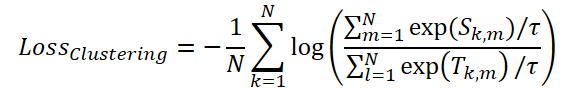
To optimize masking, the authors introduce a ClusteringLoss function.

Finally, the Time-Frequency Reconstruction Module (TFRM) applies the inverse Fourier transform (iFFT) to reconstruct the time series.

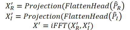
Anomalies are detected based on reconstruction error.

By using complex analysis that combines time- and frequency-domain analysis, the CATCH model provides robust and reliable anomaly detection.

A visualization of the CATCH framework is shown below.

Implementation in MQL5

After reviewing the theoretical aspects of the CATCH method, we now move on to the practical part of the article, where we implement our interpretation of the proposed approaches using MQL5.

First, it is important to note that nearly all operations in this framework are performed in the frequency domain. This is a defining feature that shapes both the data processing approach and the choice of mathematical tools.

As is well known, representing signals in the frequency domain involves complex numbers. Therefore, efficient handling of complex data, including arithmetic operations, is essential for correct system performance.

We have already addressed similar challenges while working on the ATFNet framework. At that time, we established principles for spectral data processing and developed methodological approaches that can now be reused. These previous implementations significantly simplify the implementation.

Complex Convolution Layer

We begin by designing a convolutional layer capable of working with complex values. In practice, convolutional layers are among the most effective tools for processing multivariate sequences. This is why we prioritize building this component.

As usual, we start by implementing the core algorithms on the OpenCL side. Implementing key operations at the GPU level allows us to achieve maximum parallelism, which is crucial for handling multivariate data. Unlike sequential CPU computations, GPU cores process different parts of the task simultaneously, resulting in significant speedups — both during training and in production.

The feed-forward pass is implemented in the FeedForwardComplexConv kernel. This kernel receives pointers to three data buffers along with several constants defining the data structure.

It is important to note that all buffers use the vector type float2. This choice is driven by the need to efficiently process complex numbers, where each value consists of a real and an imaginary component.

Using float2 provides several key advantages:

• Optimized memory access: vector representation allows reading and writing two values simultaneously, reducing memory operations.
• Hardware acceleration: OpenCL supports vector types at the hardware level, speeding up arithmetic computations.
• Cleaner data representation: float2 makes the code more intuitive, as each variable directly corresponds to a complex number.

__kernel void FeedForwardComplexConv(__global const float2 *matrix_w,
                                     __global const float2 *matrix_i,
                                     __global float2 *matrix_o,
                                     const int inputs,
                                     const int step,
                                     const int window_in,
                                     const int activation
                                    )
  {
   const size_t i = get_global_id(0);
   const size_t units = get_global_size(0);
   const size_t out = get_global_id(1);
   const size_t w_out = get_global_size(1);
   const size_t var = get_global_id(2);
   const size_t variables = get_global_size(2);

The kernel is designed to operate in a three-dimensional execution space. The first dimension corresponds to the number of elements in the sequence. The second dimension corresponds to the number of filters, while the third one represents the number of independent unit sequences within the overall input tensor. At the start of the kernel, we identify the current execution thread across all dimensions of this space. And we save the resulting indices in local constants.

Next, based on these indices, offsets within the data buffers are calculated. This step mirrors the logic used in the previously implemented convolutional layer for real-valued data, which is made possible by representing complex numbers with vector data types.

int w_in = window_in;
int shift_out = w_out * (i + units * var);
int shift_in = step * i + inputs * var;
int shift = (w_in + 1) * (out + var * w_out);
int stop = (w_in <= (inputs - shift_in) ? w_in : (inputs - shift_in)) + inputs * var;

This completes the preparatory stage. Now, let's proceed to the convolution operation. In this case, both the input data and the filter parameters are complex values. The result of the computation is also a complex number. All mathematical operations are performed using previously implemented functions for basic complex arithmetic.

First, we declare a local variable to store intermediate results and initialize it with the bias term of the filter.

   float2 sum = ComplexMul((float2)(1, 0), matrix_w[shift + w_in]);
#pragma unroll
   for(int k = 0; k <= stop; k ++)
      sum += IsNaNOrInf2(ComplexMul(matrix_i[shift_in + k], matrix_w[shift + k]), (float2)0);

Then, we execute a loop where the input data vector is multiplied element-wise by the corresponding filter vector, with the results accumulated in the local variable.

After that, the appropriate activation function is applied, and the final value is written to the output buffer.

   switch(activation)
     {
      case 0:
         sum = ComplexTanh(sum);
         break;
      case 1:
         sum = ComplexDiv((float2)(1, 0), (float2)(1, 0) + ComplexExp(-sum));
         break;
      case 2:
         if(sum.x < 0)
           {
            sum.x *= 0.01f;
            sum.y *= 0.01f;
           }
         break;
      default:
         break;
     }
   matrix_o[out + shift_out] = sum;
  }

The next step is to implement the backpropagation pass. Let us consider the kernel responsible for propagating the error gradient CalcHiddenGradientComplexConv. Here, we again use the vector-based representation of complex numbers. The method parameters include buffers for error gradients at the corresponding stages.

__kernel void CalcHiddenGradientComplexConv(__global const float2 * matrix_w,
                                            __global const float2 * matrix_g,
                                            __global const float2 * matrix_o,
                                            __global float2 * matrix_ig,
                                            const int outputs,
                                            const int step,
                                            const int window_in,
                                            const int window_out,
                                            const int activation,
                                            const int shift_out
                                           )
  {
   const size_t i = get_global_id(0);
   const size_t inputs = get_global_size(0);
   const size_t var = get_global_id(1);
   const size_t variables = get_global_size(1);

It is important to note that the purpose of this operation is to propagate the error gradient back to the input data, in proportion to their contribution to the model's output. This requirement leads to a change in the kernel execution space. In this implementation, a two-dimensional space is used. The first dimension corresponds to elements of the input sequence, and the second to the univariate sequence of the multivariate series.

As before, the kernel begins by identifying the current execution thread across all dimensions. The obtained indices are stored in local constants.

Next, offsets within the data buffers are computed. A key detail here is that a single input element may participate in multiple convolution operations, depending on the stride of the convolution window. As a result, the gradient must be aggregated across all such operations. To handle this, we define the ranges over which the gradient will be accumulated.

float2 sum = (float2)0;
float2 out = matrix_o[i];
int start = i - window_in + step;
start = max((start - start % step) / step, 0) + var * inputs;
int stop = (i + step - 1) / step;
if(stop > (outputs / window_out))
   stop = outputs / window_out;
stop += var * outputs;

Once the preparation is complete, a loop iterates over these ranges with the specified step, summing the gradients while taking into account the corresponding filter weights.

#pragma unroll
   for(int h = 0; h < window_out; h ++)
     {
      for(int k = start; k < stop; k++)
        {
         int shift_g = k * window_out + h;
         int shift_w = (stop - k - 1) * step + i % step + h * (window_in + 1);
         if(shift_g >= outputs || shift_w >= (window_in + 1) * window_out)
            break;
         sum += ComplexMul(matrix_g[shift_out + shift_g], matrix_w[shift_w]);
        }
     }
   sum = IsNaNOrInf2(sum, (float2)0);

The resulting value is then adjusted by the derivative of the activation function applied to the input data.

   switch(activation)
     {
      case 0:
         sum = ComplexMul(sum, (float2)1.0f - ComplexMul(out, out));
         break;
      case 1:
         sum = ComplexMul(sum, ComplexMul(out, (float2)1.0f - out));
         break;
      case 2:
         if(out.x < 0.0f)
           {
            sum.x *= 0.01f;
            sum.y *= 0.01f;
           }
         break;
      default:
         break;
     }
   matrix_ig[i] = sum;
  }

The result is stored in the corresponding element of the global data buffers.

You can find the full code for the kernels presented above in the attachment. The attachment also contains the complete code for the kernels for optimizing the trainable filter parameters, which I suggest you study independently. We will now move on to organizing the workflow on the main program side.

At this stage, we introduce a new object CNeuronComplexConvOCL. Its structure is shown below.

class CNeuronComplexConvOCL    :  public CNeuronConvOCL
  {
protected:
   //---
   virtual bool      feedForward(CNeuronBaseOCL *NeuronOCL);
   virtual bool      updateInputWeights(CNeuronBaseOCL *NeuronOCL);
   virtual bool      calcInputGradients(CNeuronBaseOCL *NeuronOCL);

public:
                     CNeuronComplexConvOCL(void)   {  activation = None;   }
                    ~CNeuronComplexConvOCL(void) {};
   virtual bool      Init(uint numOutputs, uint myIndex, COpenCLMy *open_cl,
                          uint window, uint step, uint window_out, 
                          uint units_count, uint variables, 
                          ENUM_OPTIMIZATION optimization_type, uint batch);
   //---
   virtual int       Type(void)   const   {  return defNeuronComplexConvOCL;   }
  };

This class inherits from the convolutional layer object used for real values. This allows us to reuse the existing infrastructure, including internal objects and interfaces. However, some adjustments to inherited methods are still required.

First and foremost, this applies to the feed-forward and backpropagation methods. These are overridden to work with the new OpenCL kernels described above. The process of enqueueing these kernels for execution follows the standard procedure. So we will not go into detail here. The full implementation is provided in the attachments.

That said, it is worth taking a closer look at the new object initialization method, since working with complex numbers affects how data buffers are handled. Although MQL5 does support complex numbers natively, we chose not to introduce new buffer types. Instead, we increased the size of the existing buffers. This approach keeps the solution more universal and avoids the need for extensive changes to existing methods.

The structure of the initialization method parameters is fully inherited from the parent class.

bool CNeuronComplexConvOCL::Init(uint numOutputs, uint myIndex, COpenCLMy *open_cl,
                                 uint window, uint step, uint window_out, 
                                 uint units_count, uint variables, 
                                 ENUM_OPTIMIZATION optimization_type, uint batch)
  {
   if(!CNeuronBaseOCL::Init(numOutputs, myIndex, open_cl, 2 * units_count * window_out * variables,
                                                                         optimization_type, batch))
      return false;

Inside the method, we first call the corresponding method of the fully connected layer, which serves as the base class for all neural network layers in our library, including convolutional layer. We cannot directly use the method from the immediate parent class due to differences in buffer sizes.

Note that when specifying the size of the object created via the parent method, we set it to twice the calculated size. As expected, this is necessary to store both the real and imaginary parts of complex values.

Next, we store the architecture constants of the object in internal variables.

iWindow = (int)window;
iStep = MathMax(step, 1);
activation = None;
iWindowOut = window_out;
iVariables = variables;

We then proceed to initialize the inherited data buffers. First, we check whether the buffer for trainable parameters is valid and create a new one if needed.

if(CheckPointer(WeightsConv) == POINTER_INVALID)
  {
   WeightsConv = new CBufferFloat();
   if(CheckPointer(WeightsConv) == POINTER_INVALID)
      return false;
  }

When determining the size of this buffer, we again account for complex values. We double the expected size accordingly.

int count = (int)(2 * (iWindow + 1) * iWindowOut * iVariables);
if(!WeightsConv.Reserve(count))
   return false;

The buffer is then initialized with random values.

float k = (float)(1 / sqrt(iWindow + 1));
for(int i = 0; i < count; i++)
  {
   if(!WeightsConv.Add((GenerateWeight() * 2 * k - k)*WeightsMultiplier))
    return false;
  }
if(!WeightsConv.BufferCreate(OpenCL))
   return false;

Finally, depending on the chosen optimization method, we allocate the required number of buffers for storing optimizer state momentum terms. These buffers are initially filled with zeros.

   if(optimization == SGD)
     {
      if(CheckPointer(DeltaWeightsConv) == POINTER_INVALID)
        {
         DeltaWeightsConv = new CBufferFloat();
         if(CheckPointer(DeltaWeightsConv) == POINTER_INVALID)
            return false;
        }
      if(!DeltaWeightsConv.BufferInit(count, 0.0))
         return false;
      if(!DeltaWeightsConv.BufferCreate(OpenCL))
         return false;
     }
   else
     {
      if(CheckPointer(FirstMomentumConv) == POINTER_INVALID)
        {
         FirstMomentumConv = new CBufferFloat();
         if(CheckPointer(FirstMomentumConv) == POINTER_INVALID)
            return false;
        }
      if(!FirstMomentumConv.BufferInit(count, 0.0))
         return false;
      if(!FirstMomentumConv.BufferCreate(OpenCL))
         return false;
      //---
      if(CheckPointer(SecondMomentumConv) == POINTER_INVALID)
        {
         SecondMomentumConv = new CBufferFloat();
         if(CheckPointer(SecondMomentumConv) == POINTER_INVALID)
            return false;
        }
      if(!SecondMomentumConv.BufferInit(count, 0.0))
         return false;
      if(!SecondMomentumConv.BufferCreate(OpenCL))
         return false;
     }
//---
   return true;
  }

Finally, the method completes by returning a boolean result indicating whether the operations were executed successfully.

This concludes our discussion of the convolution-layer algorithms for complex-valueв data. The full implementation of this class and all its methods is available in the attachment.

Complex Masked Attention Module

The next major component we will build is a masked attention module for complex-valued data, which forms the core of the Channel Fusion Module.

We have previously implemented masked attention mechanisms for real-valued data. Now, our task is to extend this approach to complex numbers while incorporating several key features specific to the CATCH framework.

As usual, development begins on the OpenCL side. The feed-forward pass is implemented in the MaskAttentionComplex kernel. This kernel takes pointers to five data buffers and two constants defining the structure of the input data. Since we are working with complex numbers, the buffers for input and output data use the float2 vector type. Meanwhile, the mask matrix and attention coefficients buffers still contain real values, as they represent probability distributions.

__kernel void MaskAttentionComplex(__global const float2 *q,
                                   __global const float2 *kv,
                                   __global float2 *scores,
                                   __global const float *masks,
                                   __global float2 *out,
                                   const int dimension,
                                   const int heads_kv
                                  )
  {
//--- init
   const int q_id = get_global_id(0);
   const int k = get_local_id(1);
   const int h = get_global_id(2);
   const int qunits = get_global_size(0);
   const int kunits = get_local_size(1);
   const int heads = get_global_size(2);

The kernel operates in a three-dimensional execution space. The first dimension corresponds to the size of the Query tensor and specifies the number of elements being analyzed. The second dimension corresponds to the Key tensor with the number of elements used to compute dependencies. Along this dimension, threads are grouped into workgroups. The third dimension represents the number of attention heads. At the start of execution, each thread identifies its position in this space, storing the indices in local constants.

Using these indices, offsets for all data buffers are computed.

   const int h_kv = h % heads_kv;
   const int shift_q = dimension * (q_id * heads + h);
   const int shift_k = dimension * (2 *  heads_kv * k + h_kv);
   const int shift_v = dimension * (2 *  heads_kv * k + heads_kv + h_kv);
   const int shift_s = kunits * (q_id *  heads + h) + k;

The mask value is then loaded into a local variable.

   const float mask = IsNaNOrInf(masks[shift_s], 0);

It is important to note that the kernel expects a mask tensor that already accounts for attention heads. In other words, each attention head has its own channel mask matrix.

Next, we declare an array in the local OpenCL context memory, which we will use for data exchange within the workgroup.

   const uint ls = min((uint)kunits, (uint)LOCAL_ARRAY_SIZE);
   float2 koef = (float2)(fmax((float)sqrt((float)dimension), (float)1), 0);
   __local float2 temp[LOCAL_ARRAY_SIZE];

This completes the preparatory work stage, and we move directly to the calculation operations. First, we need to compute attention coefficients. For this, we execute a loop over the corresponding Query and Key vectors. The exponential of their product is multiplied by the mask.

//--- Score
   float score = 0;
   float2 score2 = (float2)0;
   if(ComplexAbs(mask) >= 0.01)
     {
      for(int d = 0; d < dimension; d++)
         score2 = IsNaNOrInf2(ComplexMul(q[shift_q + d], kv[shift_k + d]), (float2)0);
      score = IsNaNOrInf(ComplexAbs(ComplexExp(ComplexDiv(score, koef))) * mask, 0);
     }

Note that this operation is only performed if the mask value exceeds a predefined threshold. This effectively eliminates the influence of irrelevant channels.

The resulting values must then be normalized using the SoftMax function to obtain a proper probability distribution. To do this, we sum the values across the workgroup. First, partial sums are computed within elements of the local array.

//--- sum of exp
#pragma unroll
   for(int i = 0; i < kunits; i += ls)
     {
      if(k >= i && k < (i + ls))
         temp[k % ls].x = (i == 0 ? 0 : temp[k % ls].x) + score;
      barrier(CLK_LOCAL_MEM_FENCE);
     }

Then, these partial sums are aggregated into a final total.

   uint count = ls;
#pragma unroll
   do
     {
      count = (count + 1) / 2;
      if(k < ls)
         temp[k].x += (k < count && (k + count) < kunits ? temp[k + count].x : 0);
      if(k + count < ls)
         temp[k + count].x = 0;
      barrier(CLK_LOCAL_MEM_FENCE);
     }
   while(count > 1);

After all iterations, the first element of the local array holds the total sum for the entire workgroup. Each thread then divides its attention coefficient by this sum to obtain a normalized value. The result is written to the global output buffer.

//--- score
   if(temp[0].x > 0)
      score = score / temp[0].x;
   scores[shift_s] = score;

Next, we compute the final representation of each element, taking into account contributions from other channels. This involves multiplying the vector of attention coefficients by the Value matrix. This process is complicated by the need to perform operations in parallel workgroup threads, since each thread contains only one attention coefficient. Therefore, the process requires a nested loop structure. The outer loop iterates over elements of the corresponding row in the Value matrix.

//--- out
#pragma unroll
   for(int d = 0; d < dimension; d++)
     {
      float2 val = (score > 0 ? ComplexMul(kv[shift_v + d], (float2)(score,0)) : (float2)0);

Inside the loop, each thread loads the relevant value from global memory and multiplies it by its attention coefficient, storing the result in a local variable. To reduce costly global memory access, this step is only performed when the attention coefficient is greater than zero. Otherwise, the variable is safely initialized to zero without accessing global memory.

The next step is to sum these intermediate results across threads within the workgroup. Here we use a process similar to summing the attention coefficients. First, we sum partial results in the local array.

#pragma unroll
      for(int i = 0; i < kunits; i += ls)
        {
         if(k >= i && k < (i + ls))
            temp[k % ls] = (i == 0 ? (float2)0 : temp[k % ls]) + val;
         barrier(CLK_LOCAL_MEM_FENCE);
        }

And then we sum the values of the elements of the local array.

      uint count = ls;
#pragma unroll
      do
        {
         count = (count + 1) / 2;
         if(k < ls)
            temp[k] += (k < count && (k + count) < kunits ? temp[k + count] : (float2)0);
         if((k + count) < ls)
            temp[k + count] = (float2)0;
         barrier(CLK_LOCAL_MEM_FENCE);
        }
      while(count > 1);

Only a single thread is needed to write the final result to the global buffer.

      //---
      if(k == 0)
         out[shift_q + d] = temp[0];
      barrier(CLK_LOCAL_MEM_FENCE);
     }
  }

Before moving to the next iteration, all threads in the workgroup are synchronized.

After all iterations are complete, the kernel execution ends.

The next stage is to implement backpropagation through the complex masked attention mechanism. We implement this in the MaskAttentionGradientsComplex kernel.

__kernel void MaskAttentionGradientsComplex(__global const float2 *q, __global float2 *q_g,
                                            __global const float2 *kv, __global float2 *kv_g,
                                            __global const float *scores,
                                            __global const float *mask, __global float *mask_g,
                                            __global const float2 *gradient,
                                            const int kunits, const int heads_kv
                                           )
  {
//--- init
   const int q_id = get_global_id(0);
   const int d = get_global_id(1);
   const int h = get_global_id(2);
   const int qunits = get_global_size(0);
   const int dimension = get_global_size(1);
   const int heads = get_global_size(2);

The structure of this kernel is largely similar to the feed-forward pass. We just add global buffers for storing error gradients. However, the execution space is slightly modified. It remains three-dimensional, but the second dimension now represents the size of the internal vectors, and threads are no longer grouped into workgroups.

In the kernel body, we identify the current thread across all dimensions of the task space, storing the obtained values in local constants. As before, we use them to determine offsets into global data buffers.

   const int h_kv = h % heads_kv;
   const int shift_q = dimension * (q_id * heads + h) + d;
   const int shift_s = (q_id * heads + h) * kunits;
   const int shift_g = h * dimension + d;
   float2 koef = (float2)(fmax(sqrt((float)dimension), (float)1), 0);

After completing the preparatory work, we proceed directly to collecting error gradients. First, we define the error at the Value tensor level.

Recall that the Value tensor is used to generate all elements of the output sequence via multiplication with the attention matrix. Therefore, gradients from the attention output are propagated back to the Value tensor, weighted by the corresponding attention coefficients. This is implemented through a system of loops.

//--- Calculating Value's gradients
   int step_score = kunits * heads;
   if(h < heads_kv)
     {
#pragma unroll
      for(int v = q_id; v < kunits; v += qunits)
        {
         float2 grad = (float2)0;
         for(int hq = h; hq < heads; hq += heads_kv)
           {
            int shift_score = hq * kunits + v;
            for(int g = 0; g < qunits; g++)
              {
               float sc = IsNaNOrInf(scores[shift_score + g * step_score], 0);
               if(sc > 0)
                  grad += ComplexMul(gradient[shift_g + dimension * (hq - h + g  * heads)],
                                     (float2)(sc, 0));
              }
           }
         int shift_v = dimension * (2 *  heads_kv * v + heads_kv + h) + d;
         kv_g[shift_v] = grad;
        }
     }

Next, we propagate the error gradient to the Query tensor level. Each element of the Query tensor influences only a single output element. Therefore, the corresponding gradient can be stored in a local variable to minimize global memory access.

//--- Calculating Query's gradients
   float2 grad = 0;
   float2 out_g = IsNaNOrInf2(gradient[shift_g + q_id * dimension], (float2)0);
   int shift_val = (heads_kv + h_kv) * dimension + d;
   int shift_key = h_kv * dimension + d;
#pragma unroll
   for(int k = 0; (k < kunits && ComplexAbs(out_g) != 0); k++)
     {
      float2 sc_g = 0;
      float2 sc = (float2)(scores[shift_s + k], 0);
      for(int v = 0; v < kunits; v++)
         sc_g += IsNaNOrInf2(ComplexMul(
                                ComplexMul((float2)(scores[shift_s + v], 0),
                                           out_g * kv[shift_val + 2 * v * heads_kv * dimension]),
                                ((float2)(k == v, 0) - sc)), (float2)0);
      float m = mask[shift_s + k];
      mask_g[shift_s + k] = IsNaNOrInf(sc.x / m * sc_g.x + sc.y / m * sc_g.y, 0);
      grad += IsNaNOrInf2(ComplexMul(sc_g, kv[shift_key + 2*k*heads_kv*dimension]), (float2)0);
     }
   q_g[shift_q] = IsNaNOrInf2(ComplexDiv(grad, koef), (float2)0);

However, when generating the resulting value, we interact with a whole series of Key and Value tensor values. To obtain the required error value, we first propagate the gradient to the attention coefficient matrix, and only then transfer it to the Query tensor.

Note that here we also propagate the error gradient to the channel masking matrix.

Finally, gradients are propagated to the Key tensor. The algorithm is very similar to the Query case, except that the computation proceeds along the columns of the attention matrix.

//--- Calculating Key's gradients
   if(h < heads_kv)
     {
#pragma unroll
      for(int k = q_id; k < kunits; k += qunits)
        {
         int shift_k = dimension * (2 *  heads_kv * k + h_kv) + d;
         grad = 0;
         for(int hq = h; hq < heads; hq++)
           {
            int shift_score = hq * kunits + k;
            float2 val = IsNaNOrInf2(kv[shift_k + heads_kv * dimension], (float2)0);
            for(int scr = 0; scr < qunits; scr++)
              {
               float2 sc_g = (float2)0;
               int shift_sc = scr * kunits * heads;
               float2 sc = (float2)(IsNaNOrInf(scores[shift_sc + k], 0), 0);
               if(ComplexAbs(sc) == 0)
                  continue;
               for(int v = 0; v < kunits; v++)
                  sc_g += IsNaNOrInf2(
                             ComplexMul(
                                ComplexMul((float2)(scores[shift_sc + v], 0),
                                           gradient[shift_g + scr * dimension]),
                                ComplexMul(val, ((float2)(k == v, 0) - sc))),
                             (float2)0);
               grad += IsNaNOrInf2(ComplexMul(sc_g, q[shift_q + scr * dimension]), (float2)0);
              }
           }
         kv_g[shift_k] = IsNaNOrInf2(ComplexDiv(grad, koef), (float2)0);
        }
     }
  }

This completes our overview of the algorithms for implementing complex-valued masked attention within the OpenCL environment. The full kernel implementations can be found in the attachments.

The next step will be to implement the masked attention logic on the main program side. We will cover this in the next article.

Conclusion

In this article, we explored the theoretical foundations of the CATCH framework, which combines the Fourier transform with frequency patching to detect anomalies in multivariate time series. Its key advantage lies in its ability to uncover complex market patterns that remain hidden when analyzing data solely in the time domain.

The use of frequency-domain representation provides deeper insight into market dynamics, while frequency patching adapts the analysis to changing conditions. In addition, CATCH captures relationships between assets, making it more sensitive to systemic anomalies. Unlike traditional methods, it not only detects obvious spikes and outliers but also identifies subtle, hidden dependencies that may signal upcoming shifts in market trends.

In the practical section, we began implementing our own version of the framework in MQL5. In the next article, we will continue this work and ultimately evaluate the performance of the implemented solutions on real historical data.

Related Links

• CATCH: Channel-Aware multivariate Time Series Anomaly Detection via Frequency Patching
• Other articles from this series

Programs Used in the Article

#	Name	Type	Description
1	Research.mq5	Expert Advisor	Expert Advisor for collecting datasets
2	ResearchRealORL.mq5	Expert Advisor	Expert Advisor for collecting datasets using the Real-ORL method
3	Study.mq5	Expert Advisor	Model Training Expert Advisor
4	Test.mq5	Expert Advisor	Model Testing Expert Advisor
5	Trajectory.mqh	Class Library	System state and model architecture description structure
6	NeuroNet.mqh	Class Library	A library of classes for creating a neural network
7	NeuroNet.cl	Library	OpenCL program code