
Neural Networks in Trading: Integrating Chaos Theory into Time Series Forecasting (Final Part)

Introduction
We continue developing our own vision on the approaches proposed by the authors of the Attraos framework. In the previous article, we explored the theoretical aspects of the framework. The framework applies principles of chaos theory to solve time series forecasting problems.
The architecture of the Attraos framework is a complex, multi-component system that combines methods of nonlinear analysis, machine learning, and computational optimization. The use of the Phase Space Reconstruction (PSR) method allows Attraos to model hidden dynamic processes and account for nonlinear relationships among various market variables. This enables the identification of stable structures in market data and their use to improve the accuracy of forecasts for future price movements.
One of the key features of Attraos is the Multi-Resolution Dynamic Memory Unit (MDMU), which allows the model to retain historical price movement patterns and adapt to changing market conditions. This is particularly important in financial markets, where patterns can recur across different time intervals with varying amplitude and intensity. The model dynamically adapts to the evolving structure of financial markets, providing more accurate predictions across multiple time horizons.
Applying a local evolution strategy in the frequency domain enables adaptation to changing market conditions while enhancing differences between attractors. This helps the model minimize errors and control attractor deviations, ensuring both stability and high forecast accuracy.
The original visualization of the Attraos framework is provided below.

In the practical part of the previous article, we implemented the basic components on the OpenCL side. Today, we move on to creating objects in the main program.
Constructing the Attraos Object
The Attraos algorithm begins with the PSR module, which transforms the analyzed time series into phase space according to a specified time lag. This process is a key step in data preprocessing, allowing hidden dependencies, time series structure, and latent dynamic patterns to be identified.
A multidimensional time series is usually represented as a matrix, with each row containing the parameters of the analyzed system at a given time point t. In our case, however, the data are stored in one-dimensional buffers, and the matrix representation is purely conventional. The data are organized such that vectors describing the system state at each time point are stored sequentially in the buffer. The size of each vector is determined by the window parameter. Consequently, to create subsequences with a given time lag, it is sufficient to proportionally increase the window value while reducing the sequence length. Thus, the transformation of a time series into phase space requires no additional computational resources and is implemented solely through the model architecture design.
All subsequent operations of the framework are structured within the CNeuronAttraos object, whose structure is outlined below.
class CNeuronAttraos :  public CNeuronBaseOCL
  {
protected:
   CNeuronBaseOCL    cOne;
   CNeuronBaseOCL    cX_norm;
   CNeuronConvOCL    cA;
   CNeuronConvOCL    cX_proj;
   CNeuronBaseOCL    cDelta;
   CNeuronBaseOCL    cB;
   CNeuronBaseOCL    cC;
   CNeuronConvOCL    cD;
   CNeuronBaseOCL    cH;
   CNeuronConvOCL    cDelta_proj;
   CNeuronBaseOCL    cDeltaA;
   CNeuronBaseOCL    cDeltaB;
   CNeuronBaseOCL    cDeltaBX;
   CNeuronBaseOCL    cDeltaH;
   CNeuronBaseOCL    cHS;
   //---
   virtual bool      PScan(void);
   virtual bool      PScanCalcGradient(void);
   //---
   virtual bool      feedForward(CNeuronBaseOCL *NeuronOCL) override;
   virtual bool      updateInputWeights(CNeuronBaseOCL *NeuronOCL) override;
   virtual bool      calcInputGradients(CNeuronBaseOCL *NeuronOCL) override;

public:
                     CNeuronAttraos(void) {};
                    ~CNeuronAttraos(void) {};
   //---
   virtual bool      Init(uint numOutputs, uint myIndex, COpenCLMy *open_cl,
                          uint window, uint window_key, uint units_count,
                          ENUM_OPTIMIZATION optimization_type, uint batch);
   //---
   virtual int       Type(void) override   const   {  return defNeuronAttraos; }
   //---
   virtual bool      Save(int const file_handle) override;
   virtual bool      Load(int const file_handle) override;
   //---
   virtual bool      WeightsUpdate(CNeuronBaseOCL *source, float tau) override;
   virtual void      SetOpenCL(COpenCLMy *obj) override;
  };
In this new class structure, in addition to the standard set of overridable virtual methods, we observe a significant number of internal objects. They perform different functions and facilitate interaction among the class elements. Using internal objects allows for more efficient code organization. Each object is responsible for a specific task, making the system modular and easier to modify. During implementation of the new object's methods, we will examine the functionality of each internal component in detail to understand its purpose and role in the overall structure.
All internal objects are declared as static, eliminating the need for dynamic creation and deletion. Consequently, the class constructor and destructor remain empty, as memory management for these objects is automatic. The initialization of these declared and inherited objects is performed in the Init method. The method receives constants as parameters to uniquely define the architecture of the object being created. The structure of these parameters should be self-explanatory.
bool CNeuronAttraos::Init(uint numOutputs, uint myIndex, COpenCLMy *open_cl,
                       uint window, uint window_key, uint units_count,
                       ENUM_OPTIMIZATION optimization_type, uint batch)
  {
   if(!CNeuronBaseOCL::Init(numOutputs, myIndex, open_cl, window * units_count, optimization_type, batch))
      return false;
   SetActivationFunction(None);
In the method body, the parent class’s identically named method is called first. This method sets up minimal control points and initializes inherited interfaces.
We explicitly disable the activation function for our object at this stage, as all processes are handled via internal objects. Inherited interfaces are used solely for global-level data exchange.
After the parent class method executes successfully, we proceed to initialize the declared objects. Initially, we initialize objects for two matrices of trainable parameters:
- A — the state transition matrix
- D — the matrix of residual connections with the original data
Since these matrices will be multiplied by full matrices containing all elements of the analyzed sequence, their values must immediately be repeated across the number of sequence elements. This avoids additional copy operations and optimizes the backpropagation process.
As before, we organize trainable parameters using a small two-layer model. The first layer contains fixed values, and the second generates the required tensor by multiplying internal trainable parameters by the fixed values from the first layer. This approach allows existing neural layer algorithms to train parameters without creating additional functionality. To minimize the number of trainable parameters in the second layer, the first layer typically contains only one element.
In this case, however, the output of the second layer must be a tensor with repeated values. To achieve this, the fixed values in the first layer are repeated a specified number of times. The second layer is implemented as a convolutional layer, with the number of filters equal to the number of trainable parameters. The convolution window size and stride are set to 1 so that each output tensor element depends on a single input value.
   int index = 0;
   if(!cOne.Init(0, index, OpenCL, units_count, optimization, iBatch))
      return false;
   if(!cOne.getOutput().Fill(1))
      return false;
   cOne.SetActivationFunction(None);
//---
   index++;
   if(!cA.Init(0, index, OpenCL, 1, 1, window * window_key, units_count, 1, optimization, iBatch))
      return false;
   cA.SetActivationFunction(MinusSoftPlus);
   CBufferFloat *w = cA.GetWeightsConv();
   if(!w || !w.Fill(0))
      return false;
Since the first layer contains no trainable parameters, it can also generate the second trainable parameter matrix. Hence, we initialize only the second object for generating trainable parameters.
   index++;
   if(!cD.Init(0, index, OpenCL, 1, 1, window, units_count, 1, optimization, iBatch))
      return false;
   cD.SetActivationFunction(None);
   w = cD.GetWeightsConv();
   if(!w || !w.Fill(1))
      return false;
Note that during object initialization, the trainable parameter matrices are filled with fixed values. This is somewhat different from the general approach of filling the trainable parameters with random values. Fixed initialization is useful when the model must preserve certain properties at early training stages or when initial conditions strongly influence the final parameter distribution. Here, it prevents sharp initial fluctuations and promotes smoother adaptation to the data.
The remaining state-space model parameters are generated dependent on the input data, allowing them to adapt to the specific features of the analyzed sequence. A convolutional layer generates all model entities in parallel. This approach ensures efficient data processing and significantly accelerates computations, as convolution is performed in parallel throughout the entire sequence.
Before generating the state-space model parameters, the inputs are normalized. Normalization removes scale differences in the raw values, making the optimization process smoother and more predictable.
//---
   index++;
   if(!cX_norm.Init(0, index, OpenCL, window * units_count, optimization, iBatch))
      return false;
   cX_norm.SetActivationFunction(None);
   index++;
   if(!cX_proj.Init(0, index, OpenCL, window, window, 4 * window_key, units_count, 1, optimization, iBatch))
      return false;
   cX_proj.SetActivationFunction(None);
Next, the generated model parameters are divided into individual entities. And additional objects are created for storage, with names reflecting the stored data.
   index++;
   if(!cDelta.Init(0, index, OpenCL, window_key * units_count, optimization, iBatch))
      return false;
   cDelta.SetActivationFunction(None);
   index++;
   if(!cB.Init(0, index, OpenCL, window_key * units_count, optimization, iBatch))
      return false;
   cB.SetActivationFunction(None);
   index++;
   if(!cC.Init(0, index, OpenCL, window_key * units_count, optimization, iBatch))
      return false;
   cC.SetActivationFunction(None);
   index++;
   if(!cH.Init(0, index, OpenCL, window_key * units_count, optimization, iBatch))
      return false;
   cH.SetActivationFunction(None);
We then initialize the object responsible for generating the exponential decay parameters of the hidden states. This component is critical for managing the information dynamics through the sequence, controlling the degree of retention or decay of past states.
   index++;
   if(!cDelta_proj.Init(0, index, OpenCL, window_key, window_key, window, units_count, 1, optimization, iBatch))
      return false;
   cDelta_proj.SetActivationFunction(SoftPlus);
Using SoftPlus as the activation function ensures that only positive values appear at the output.
Several additional objects are initialized to store intermediate computation results, all of equal size.
   index++;
   if(!cDeltaA.Init(0, index, OpenCL, window * window_key * units_count, optimization, iBatch))
      return false;
   cDeltaA.SetActivationFunction(None);
   index++;
   if(!cDeltaB.Init(0, index, OpenCL, window * window_key * units_count, optimization, iBatch))
      return false;
   cDeltaB.SetActivationFunction(None);
   index++;
   if(!cDeltaBX.Init(0, index, OpenCL, window * window_key * units_count, optimization, iBatch))
      return false;
   cDeltaBX.SetActivationFunction(None);
   index++;
   if(!cDeltaH.Init(0, index, OpenCL, window * window_key * units_count, optimization, iBatch))
      return false;
   cDeltaH.SetActivationFunction(None);
   index++;
   if(!cHS.Init(0, index, OpenCL, window * window_key * units_count, optimization, iBatch))
      return false;
   cHS.SetActivationFunction(None);
//---
   return true;
  }
The initialization method concludes by returning a logical result to the calling program.
Note that in this object, architecture parameters are not stored in separate local variables. This implementation avoids maintaining persistent duplicates of values already stored in internal objects. Instead, local variables are filled at the beginning of feed-forward and backpropagation methods.
After object initialization, we proceed to the forward pass algorithm, implemented in the feedForward method, which receives a pointer to the input data object.
bool CNeuronAttraos::feedForward(CNeuronBaseOCL *NeuronOCL)
  {
//---
   uint window = cX_proj.GetWindow();
   uint window_key = cX_proj.GetFilters() / 4;
   uint units = cD.GetUnits();
In the method body, we first load parameters from internal objects that were not stored during initialization. Then we generate tensors for the trainable parameters of the model.
   if(!cA.FeedForward(cOne.AsObject()))   // (Units, Window, WindowKey)
      return false;
   if(!cD.FeedForward(cOne.AsObject()))   // (Units, Window))
      return false;
Next, we normalize the input data and generate context-dependent model parameters.
   if(!NeuronOCL ||
      !SumAndNormilize(NeuronOCL.getOutput(), NeuronOCL.getOutput(), cX_norm.getOutput(), window, true, 0, 0, 0, 0.5f))
      return false;
   if(!cX_proj.FeedForward(cX_norm.AsObject()))    // (Units, 4*WindowKey)
      return false;
They are then separated into individual entities.
   if(!DeConcat(cDelta.getOutput(), cB.getOutput(), cC.getOutput(), cH.getOutput(), cX_proj.getOutput(),
                window_key, window_key, window_key, window_key, units))   // 4*(Units, WindowKey)
      return false;
We also generate adaptive time-step parameters.
   if(!cDelta_proj.FeedForward(cDelta.AsObject()))       // (Units, Window)
      return false;
At this point, the preparatory stage is complete, and we proceed to constructing the MDMU algorithm, responsible for modeling the time series dynamics. The model state is updated according to the recurrent equation:
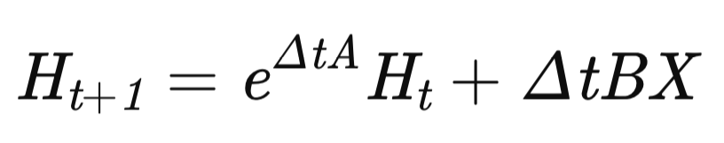
where Δt is the adaptive time step.
Initially, we calculate the exponential component in the first term, replacing the standard exponential function with SoftPlus, which offers several advantages.
   if(!DiagMatMul(cDelta_proj.getOutput(), cA.getOutput(), cDeltaA.getOutput(),
                  window, window_key, units, SoftPlus))  // (Units, Window, WindowKey)
      return false;
SoftPlus grows more slowly than the exponential, reducing the risk of sharp increases in the transition matrix. This ensures smoother gradient changes and more stable training.
The exponential function is highly sensitive to small Δ changes. SoftPlus smooths variations, preventing abrupt jumps in hidden states.
In noisy data, SoftPlus limits the impact of outliers, as its growth is constrained logarithmically, enhancing model stability.
Next, the values of the second term are calculated by sequential matrix multiplications.
   if(!MatMul(cDelta_proj.getOutput(), cB.getOutput(), cDeltaB.getOutput(),
              window, 1, window_key, units))             // (Units, Window, WindowKey)
      return false;
   if(!DiagMatMul(cX_norm.getOutput(), cDeltaB.getOutput(), cDeltaBX.getOutput(),
                  window, window_key, units, None))      // (Units, Window, WindowKey)
      return false;
We then adjust the dynamic regulator matrix for changes in hidden states according to the rate of change of the hidden state.
   if(!MatMul(cDelta_proj.getOutput(), cH.getOutput(), cDeltaH.getOutput(),
              window, 1, window_key, units))             // (Units, Window, WindowKey)
      return false;
After preparing all necessary data, we correct the system’s hidden states using the parallel scan algorithm implemented in the previous article on the OpenCL side. Here, it is sufficient to call the PScan kernel wrapper.
if(!PScan())
   return false;
The kernel invocation follows a standard algorithm, so we will not examine it in detail here. The complete code for this method is included in the attachment (file NeuroNet.cl).
Next, we generate the forecasted state of the analyzed system by multiplying the updated hidden state matrix by the hidden state projection matrix.
if(!MatMul(cHS.getOutput(), cC.getOutput(), Output, window, window_key, 1, units)) // (Units, Window, 1)
   return false;
Normalized input data are multiplied by the direct connection coefficients.
if(!ElementMult(cD.getOutput(), cX_norm.getOutput(), PrevOutput))           // (Units, Window))
   return false;
The results of the two operations are then summed.
if(!SumAndNormilize(Output, PrevOutput, Output, window, false, 0, 0, 0, 1))   // (Units, Window))
   return false;
Additionally, we incorporate the original input data by creating a residual connection path.
   if(!SumAndNormilize(Output, NeuronOCL.getOutput(), Output, window, false, 0, 0, 0, 1))   // (Units, Window))
      return false;
//---
   return true;
  }
This approach integrates information from hidden states and short-term dependencies in the input data.
This completes the forward pass algorithm of our Attraos framework implementation. Then we return the logical result of the operation to the caller and complete the method execution.
The next step is constructing the backward pass algorithms for our object. In this article, we examine the calcInputGradients method, which distributes error gradients. Like before, the method receives a pointer to the input data object, but this time it also takes the error size according to the influence of the input data on the final model output.
bool CNeuronAttraos::calcInputGradients(CNeuronBaseOCL *NeuronOCL)
  {
   if(!NeuronOCL)
      return false;
The method first checks the validity of the pointer. If the pointers are invalid or outdated, any further operations would be meaningless.
We then save input data parameters in local variables as in the forward pass.
uint window = cX_proj.GetWindow();
uint window_key = cX_proj.GetFilters() / 4;
uint units = cD.GetUnits();
Next, we distribute the error gradient from the output level across the three data streams. Let me remind you that during the feed-forward pass we used 3 data transfer information flows:
- State-space model
- Direct connections with coefficients
- Residual connections
First, the error gradient is distributed between direct connection coefficients and normalized input data.
if(!ElementMultGrad(cD.getOutput(), cD.getGradient(), cX_norm.getOutput(), cX_norm.getPrevOutput(),
                    Gradient, cD.Activation(), None))          // (Units, Window))
   return false;
Next, the gradient is propagated along the second data stream, distributing it between hidden states and projection coefficients.
if(!MatMulGrad(cHS.getOutput(), cHS.getGradient(), cC.getOutput(), cC.getGradient(), Gradient,
               window, window_key, 1, units)) // (Units, Window, 1)
   return false;
If necessary, results are corrected using derivatives of the corresponding activation functions.
if(cHS.Activation() != None)
  {
   if(!DeActivation(cHS.getOutput(), cHS.getGradient(), cHS.getGradient(), cHS.Activation()))
      return false;
  }
if(cC.Activation() != None)
  {
   if(!DeActivation(cC.getOutput(), cC.getGradient(), cC.getGradient(), cC.Activation()))
      return false;
  }
We then distribute the gradient through the parallel scan module using the corresponding kernel wrapper.
if(!PScanCalcGradient())
   return false;
The resulting values are assigned to the appropriate entities. First, the gradient is passed to hidden states and adaptive time-step parameters.
if(!MatMulGrad(cDelta_proj.getOutput(), cDelta_proj.getGradient(), cH.getOutput(), cH.getGradient(),
               cDeltaH.getGradient(), window, 1, window_key, units))             // (Units, Window, WindowKey)
   return false;
Then the error gradient is propagated to normalized input data.
if(!DiagMatMulGrad(cX_norm.getOutput(), cX_norm.getGradient(), cDeltaB.getOutput(), cDeltaB.getGradient(),
                   cDeltaBX.getGradient(), window, window_key, units))      // (Units, Window, WindowKey)
   return false;
if(!SumAndNormilize(cX_norm.getGradient(), cX_norm.getPrevOutput(), cX_norm.getPrevOutput(),
                                                                  window, false, 0, 0, 0, 1))
   return false;
Note that we have already passed the error gradient values into the normalized input object. Therefore, at this stage, we summarize the data from the two information streams.
Similarly, gradients are distributed to the coefficients controlling input influence on hidden states and adaptive time-step parameters.
if(!MatMulGrad(cDelta_proj.getOutput(), cDelta_proj.getPrevOutput(), cB.getOutput(), cB.getGradient(),
               cDeltaB.getGradient(), window, 1, window_key, units))             // (Units, Window, WindowKey)
   return false;
if(!SumAndNormilize(cDelta_proj.getGradient(), cDelta_proj.getPrevOutput(), cDelta_proj.getGradient(),
                    window, false, 0, 0, 0, 1))
   return false;
Gradients for adaptive time-step parameters are accumulated with previously collected values.
Next, the error gradient is propagated to the hidden state evolution matrix, with values corrected using the derivative of the activation function.
if(!DeActivation(cDeltaA.getOutput(), cDeltaA.getGradient(), cDeltaA.getGradient(), SoftPlus))
   return false;
Then we distribute the values between the entities.
if(!DiagMatMulGrad(cDelta_proj.getOutput(), cDelta_proj.getPrevOutput(), cA.getOutput(), cA.getGradient(),
                   cDeltaA.getGradient(), window, window_key, units))  // (Units, Window, WindowKey)
   return false;
if(!SumAndNormilize(cDelta_proj.getGradient(), cDelta_proj.getPrevOutput(), cDelta_proj.getGradient(),
                    window, false, 0, 0, 0, 1))
   return false;
At this stage, we again sum the error gradient values at the adaptive time step parameter level. However, this time, this is the last information stream in this direction. Then, we adjust the accumulated values by the derivative of the corresponding activation function.
if(cDelta_proj.Activation() != None)
  {
   if(!DeActivation(cDelta_proj.getOutput(), cDelta_proj.getGradient(), cDelta_proj.getGradient(),
                                                                        cDelta_proj.Activation()))
      return false;
  }
After that we propagate the error gradient to the level of adaptive time steps.
if(!cDelta.calcHiddenGradients(cDelta_proj.AsObject()))
   return false;
At this stage, we have obtained error gradients for all context-dependent entities. These values are collected into a single tensor.
if(!Concat(cDelta.getGradient(), cB.getGradient(), cC.getGradient(), cH.getGradient(), cX_proj.getGradient(),
           window_key, window_key, window_key, window_key, units))   // 4*(Units, WindowKey)
   return false;
The error gradient is then propagated down to the level of normalized input data.
if(!cX_norm.calcHiddenGradients(cX_proj.AsObject()))
   return false;
if(!SumAndNormilize(cX_norm.getGradient(), cX_norm.getPrevOutput(), cX_norm.getGradient(),
                                                               window, false, 0, 0, 0, 1))
   return false;
Recall that the normalized input data object has already received the error gradient twice. Therefore, the values obtained at this stage are added to the previously accumulated gradients.
We also incorporate values from the residual connection path before passing the accumulated gradients to the input data level, adjusting them by the derivative of the corresponding activation function.
   if(!SumAndNormilize(cX_norm.getGradient(), Gradient, cX_norm.getGradient(), window, false, 0, 0, 0, 1))
      return false;
   if(!DeActivation(NeuronOCL.getOutput(), NeuronOCL.getGradient(), cX_norm.getGradient(), NeuronOCL.Activation()))
      return false;
//---
   return true;
  }
This concludes the calcInputGradients method, which returns a logical result to the calling program.
As for the updateInputWeights method responsible for updating the model's parameters, I suggest reviewing it independently. It simply calls the corresponding update methods for the four internal objects containing trainable parameters.
I'd like to say a few words about the algorithms of the methods that save and restore object states. Our new class contains a significant number of internal objects, but only four of them hold trainable parameters. Therefore, when saving, it is sufficient to record only these four objects to disk.
bool CNeuronAttraos::Save(const int file_handle)
  {
   if(!CNeuronBaseOCL::Save(file_handle))
      return false;
//---
   if(!cA.Save(file_handle))
      return false;
   if(!cD.Save(file_handle))
      return false;
   if(!cX_proj.Save(file_handle))
      return false;
   if(!cDelta_proj.Save(file_handle))
      return false;
//---
   return true;
  }
But the question arises of how to restore the object functionality. In the Load method, previously saved data are first read from disk.
bool CNeuronAttraos::Load(const int file_handle)
  {
   if(!CNeuronBaseOCL::Load(file_handle))
      return false;
//---
   if(!LoadInsideLayer(file_handle, cA.AsObject()))
      return false;
   if(!LoadInsideLayer(file_handle, cD.AsObject()))
      return false;
   if(!LoadInsideLayer(file_handle, cX_proj.AsObject()))
      return false;
   if(!LoadInsideLayer(file_handle, cDelta_proj.AsObject()))
      return false;
Architecture parameters are then saved to local variables.
   uint window = cX_proj.GetWindow();
   uint window_key = cX_proj.GetFilters() / 4;
   uint units_count = cD.GetUnits();
The remaining algorithm mirrors the initialization process of the temporary storage objects.
   if(!cOne.Init(0, 0, OpenCL, units_count, optimization, iBatch))
      return false;
   if(!cOne.getOutput().Fill(1))
      return false;
   cOne.SetActivationFunction(None);
   int index = 3;
   if(!cX_norm.Init(0, index, OpenCL, window * units_count, optimization, iBatch))
      return false;
   cX_norm.SetActivationFunction(None);
   index += 2;
   if(!cDelta.Init(0, index, OpenCL, window_key * units_count, optimization, iBatch))
      return false;
   cDelta.SetActivationFunction(None);
   index++;
   if(!cB.Init(0, index, OpenCL, window_key * units_count, optimization, iBatch))
      return false;
   cB.SetActivationFunction(None);
   index++;
   if(!cC.Init(0, index, OpenCL, window_key * units_count, optimization, iBatch))
      return false;
   cC.SetActivationFunction(None);
   index++;
   if(!cH.Init(0, index, OpenCL, window_key * units_count, optimization, iBatch))
      return false;
   cH.SetActivationFunction(None);
   index += 2;
   if(!cDeltaA.Init(0, index, OpenCL, window * window_key * units_count, optimization, iBatch))
      return false;
   cDeltaA.SetActivationFunction(None);
   index++;
   if(!cDeltaB.Init(0, index, OpenCL, window * window_key * units_count, optimization, iBatch))
      return false;
   cDeltaB.SetActivationFunction(None);
   index++;
   if(!cDeltaBX.Init(0, index, OpenCL, window * window_key * units_count, optimization, iBatch))
      return false;
   cDeltaBX.SetActivationFunction(None);
   index++;
   if(!cDeltaH.Init(0, index, OpenCL, window * window_key * units_count, optimization, iBatch))
      return false;
   cDeltaH.SetActivationFunction(None);
   index++;
   if(!cHS.Init(0, index, OpenCL, window * window_key * units_count, optimization, iBatch))
      return false;
   cHS.SetActivationFunction(None);
//---
   return true;
  }
This approach optimizes data saving, object restoration, and disk space usage.
With this, we conclude the discussion of constructing the Attraos framework in MQL5. The full code for the CNeuronAttraos class and all its methods is included in the attachment.
Model Architecture
After implementing the Attraos framework algorithms, let's describe the architecture of the trainable models. In this experiment, two models are trained using multi-task learning. The architectures are defined in the CreateDescriptions method, which receives pointers to two dynamic arrays where the model architecture descriptions are stored.
bool CreateDescriptions(CArrayObj *&actor, CArrayObj *&probability)
  {
//---
   CLayerDescription *descr;
//---
   if(!actor)
     {
      actor = new CArrayObj();
      if(!actor)
         return false;
     }
   if(!probability)
     {
      probability = new CArrayObj();
      if(!probability)
         return false;
     }
Within the method, we first check the validity of the pointers and create new object instances if necessary.
The first model described is the actor, which uses the previously implemented Attraos approaches. As usual, the model starts with a fully connected input layer followed by batch normalization. This allows raw data from the trading terminal to be fed directly into the model. In this case, their primary normalization is performed internally by the model.
//--- Actor
   actor.Clear();
//--- Input layer
   if(!(descr = new CLayerDescription()))
      return false;
   descr.type = defNeuronBaseOCL;
   int prev_count = descr.count = (HistoryBars * BarDescr);
   descr.activation = None;
   descr.optimization = ADAM;
   if(!actor.Add(descr))
     {
      delete descr;
      return false;
     }
//--- layer 1
   if(!(descr = new CLayerDescription()))
      return false;
   descr.type = defNeuronBatchNormOCL;
   descr.count = prev_count;
   descr.batch = 1e4;
   descr.activation = None;
   descr.optimization = ADAM;
   if(!actor.Add(descr))
     {
      delete descr;
      return false;
     }
Next we use the first layer of the Attraos architecture. It transforms the input into phase space using a 5-step time lag, corresponding to 5 minutes on a 1-minute timeframe.
//--- layer 2
   if(!(descr = new CLayerDescription()))
      return false;
   descr.type = defNeuronAttraos;
   descr.window = BarDescr*5;    // 5 min
   descr.count = HistoryBars/5;  // 24
   descr.window_out = 256;
   descr.batch = 1e4;
   descr.activation = None;
   descr.optimization = ADAM;
   if(!actor.Add(descr))
     {
      delete descr;
      return false;
     }
The second layer increases the lag to 15 steps.
//--- layer 3
   if(!(descr = new CLayerDescription()))
      return false;
   descr.type = defNeuronAttraos;
   descr.window = BarDescr*15;    // 15 min
   descr.count = HistoryBars/15;  // 8
   descr.window_out = 256;
   descr.batch = 1e4;
   descr.activation = None;
   descr.optimization = ADAM;
   if(!actor.Add(descr))
     {
      delete descr;
      return false;
     }
And the third layer increases it to 30 steps.
//--- layer 4
   if(!(descr = new CLayerDescription()))
      return false;
   descr.type = defNeuronAttraos;
   descr.window = BarDescr*30;    // 30 min
   descr.count = HistoryBars/30;  // 4
   descr.window_out = 256;
   descr.batch = 1e4;
   descr.activation = None;
   descr.optimization = ADAM;
   if(!actor.Add(descr))
     {
      delete descr;
      return false;
     }
It is important to note that the output of each CNeuronAttraos object matches the dimensionality of the input data. Therefore, the next convolutional layer reduces tensor dimensionality by a factor of three.
//--- layer 5
   if(!(descr = new CLayerDescription()))
      return false;
   descr.type = defNeuronConvOCL;
   prev_count=descr.count = HistoryBars/3;
   descr.window = BarDescr*3;
   descr.step = descr.window;
   int prev_window=descr.window_out = BarDescr;
   descr.activation = SoftPlus;
   descr.optimization = ADAM;
   if(!actor.Add(descr))
     {
      delete descr;
      return false;
     }
This is followed by the decision making head, composed of three consecutive fully connected layers.
//--- layer 6
   if(!(descr = new CLayerDescription()))
      return false;
   descr.type = defNeuronBaseOCL;
   descr.count = 512;
   descr.batch = 1e4;
   descr.activation = TANH;
   descr.optimization = ADAM;
   if(!actor.Add(descr))
     {
      delete descr;
      return false;
     }
//--- layer 7
   if(!(descr = new CLayerDescription()))
      return false;
   descr.type = defNeuronBaseOCL;
   descr.count = 256;
   descr.activation = TANH;
   descr.batch = 1e4;
   descr.optimization = ADAM;
   if(!actor.Add(descr))
     {
      delete descr;
      return false;
     }
//--- layer 8
   if(!(descr = new CLayerDescription()))
      return false;
   descr.type = defNeuronBaseOCL;
   prev_count = descr.count = NActions;
   descr.activation = SoftPlus;
   descr.batch = 1e4;
   descr.optimization = ADAM;
   if(!actor.Add(descr))
     {
      delete descr;
      return false;
     }
The resulting output is normalized.
//--- layer 9
   if(!(descr = new CLayerDescription()))
      return false;
   descr.type = defNeuronBatchNormOCL;
   descr.count = prev_count;
   descr.batch = 1e4;
   descr.activation = None;
   descr.optimization = ADAM;
   if(!actor.Add(descr))
     {
      delete descr;
      return false;
     }
A risk management block is then added.
//--- layer 10
   if(!(descr = new CLayerDescription()))
      return false;
   descr.type = defNeuronMacroHFTvsRiskManager;
//--- Windows
     {
      int temp[] = {3, 15, NActions, AccountDescr}; //Window, Stack Size, N Actions, Account Description
      if(ArrayCopy(descr.windows, temp) < int(temp.Size()))
         return false;
     }
   descr.count = 10;
   descr.window_out = 16;
   descr.step = 4;                              // Heads
   descr.batch = 1e4;
   descr.activation = None;
   descr.optimization = ADAM;
   if(!actor.Add(descr))
     {
      delete descr;
      return false;
     }
//--- layer 11
   if(!(descr = new CLayerDescription()))
      return false;
   descr.type = defNeuronConvOCL;
   descr.count = NActions / 3;
   descr.window = 3;
   descr.step = 3;
   descr.window_out = 3;
   descr.activation = SIGMOID;
   descr.optimization = ADAM;
   if(!actor.Add(descr))
     {
      delete descr;
      return false;
     }
The directional probability model for predicting future movement is fully inherited from previous work without modifications. Its description is omitted here. A complete architectural description of the trainable models is provided in the attachment, including the environment interaction programs, also carried over unchanged from prior work.
Testing
Over the course of two articles, we performed significant work adapting and extending the ideas of the Attraos framework. We now reach a key stage: evaluating the functionality and effectiveness of the implemented methods on real historical data. This process is important for assessing the model's practical applicability and its ability to identify patterns, producing stable results under varying market conditions.
The model was trained on historical EURUSD M1 data for the entire year of 2024. All indicator parameters remained at default values, without additional optimization. This approach eliminates external factors such as parameter tuning to specific historical data, allowing focus on the fundamental performance of the model. Using unchanged indicator parameters also evaluates the model's ability to adapt to real market dynamics without constant intervention or reconfiguration.
Model training is performed in two stages. The first stage uses a batch size of 1, allowing each training iteration to sample a completely random state from the training set. This maximizes the model's exposure to new states. However, this alone is insufficient for correctly training the risk management block. Therefore, in the second stage, the batch size is increased to 60, allowing the model and risk management block to adjust over 60 consecutive environmental states, which corresponds to one hour on a 1-minute timeframe.
Testing used data from January–February 2025. This period was chosen to ensure a rigorous evaluation on previously unseen data. All other experimental parameters remained unchanged to ensure reproducibility and a fair comparison. This methodology eliminates random factors and allows objective assessment of algorithm performance.
The testing results are presented below.


During testing, the model executed 287 trades, with nearly 39% closed profitably. Despite the relatively low win rate, the strategy produced a positive overall result due to the profit-to-loss ratio. Specifically, the average profit per winning trade was twice the average loss, compensating for less successful trades and yielding an overall positive outcome, with a profit factor of 1.15.
The average position holding time exceeded 2 hours, indicating a tendency for short- and medium-term decisions. Notably, the longest-held position lasted nearly two days. This fact requires further analysis.
Conclusion
We explored the Attraos framework, which uses chaos theory concepts for time series forecasting. The framework integrates nonlinear analysis, phase space reconstruction, multi-resolution dynamic memory, and adaptive algorithms. These technologies enable more accurate forecasts and adaptive trading models.
In the practical section, we implemented our interpretation of these approaches in MQL5, building and training models on historical data. Testing on out-of-sample data demonstrates the model’s ability to generate profits on unseen data. However, the results also revealed some problems. In particular, we see prolonged position holding. Also, a balance curve is less smooth than desired. These results indicate potential but also highlight the need for further optimization.
It is important to note that these conclusions are specific to this implementation. The original Attraos version was not tested in this article.
List of references
- Attractor Memory for Long-Term Time Series Forecasting: A Chaos Perspective
- Other articles from this series
Programs Used in the Article
| # | Name | Type | Description |
|---|---|---|---|
| 1 | Research.mq5 | Expert Advisor | Expert Advisor for collecting samples |
| 2 | ResearchRealORL.mq5 | Expert Advisor | Expert Advisor for collecting samples using the Real-ORL method |
| 3 | Study.mq5 | Expert Advisor | Model training Expert Advisor |
| 4 | Test.mq5 | Expert Advisor | Model Testing Expert Advisor |
| 5 | Trajectory.mqh | Class library | System state and model architecture description structure |
| 6 | NeuroNet.mqh | Class library | A library of classes for creating a neural network |
| 7 | NeuroNet.cl | Code library | OpenCL program code |
Translated from Russian by MetaQuotes Ltd.
Original article: https://www.mql5.com/ru/articles/17371
Warning: All rights to these materials are reserved by MetaQuotes Ltd. Copying or reprinting of these materials in whole or in part is prohibited.
This article was written by a user of the site and reflects their personal views. MetaQuotes Ltd is not responsible for the accuracy of the information presented, nor for any consequences resulting from the use of the solutions, strategies or recommendations described.

- Free trading apps
- Over 8,000 signals for copying
- Economic news for exploring financial markets
You agree to website policy and terms of use