Neural networks made easy (Part 20): Autoencoders

MetaTrader 5 — Trading systems | 29 September 2022, 11:43

3 168

Dmitriy Gizlyk

Introduction

We continue to study unsupervised learning methods. In previous articles, we have already analyzed clustering, data compression, and association rule mining algorithms. But the previously considered unsupervised algorithms do not use neural networks. In this article, we get back to studying neural networks. This time we will take a look at Autoencoders.

1. Autoencoder architecture

Before proceeding to the description of the autoencoder architecture, let's take a look back at neural network training methods with supervised learning algorithms. When studying the algorithms, we used pairs of labeled data consisting of the pattern and the target result. We were optimizing weights so as to minimize errors between the neural network operation result and the target value.

What can a neural network learn in this case? It will learn exactly what we expect from her. That is, it will find the features that affect the target result. However, the network will give zero weight to the features that do not affect the target result or whose effect is insignificant. So, the model is trains in quite a narrow, defined direction. There is nothing wrong with that. The model perfectly does what we want from it.

But there is another side of the coin. We have already come across the concept of Transfer Learning which implies the use of a pre-trained model to solve new problems. In this case, good results will only be obtained if the previous and new target values depend on the same features. Otherwise, the model performance can be affected by the missing features which were zeroed at the previous training stage.

How will this affect task solution? Our world is not static, and it is constantly changing. Today's market drivers can lose their influence tomorrow. The market will be driven by other forces. This limits the lifetime of our model. This is quite obvious. For example, traders review their strategies from time to time. This is also confirmed by the profitability of algorithmic trading robots built using classical strategy describing methods.

When starting to study neural networks, we expected that the use of artificial intelligence would extend the model lifetime. Furthermore, by performing additional training from time to time, we would be able to generate profits for a very long rime.

To minimize the risks associated with the above property, we will use representation or feature learning, one of the areas of unsupervised learning. Representation learning combines a set of algorithms which automatically extract features from raw input data. Clustering and dimensionality reduction algorithms we considered earlier also refer to representation learning. We used linear transformations in those algorithms. Autoencoders enable studying of more complex forms.

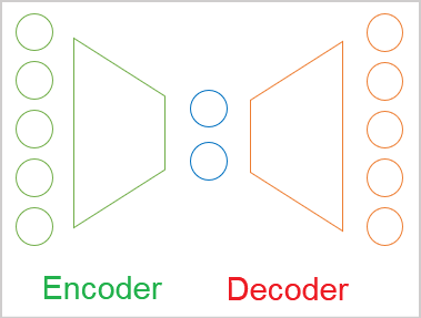
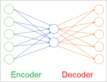
In the general case, the autoencoder is a neural network consisting of two encoder and decoder blocks. The encoder source data layer and the decoder result layer contain the same number of elements. Between them, there is a hidden layer which is usually smaller than the source data. During the learning process, the neurons of this layer form a latent (hidden) state which can describe the source data in a compressed form.

This is similar to the data compression problem we solved using the Principal Component Analysis method. However, there are differences in the approaches which we will discuss later.

As mentioned above, an autoencoder is a neural network. It is trained by the backpropagation method. The trick is that since we use unlabeled data, we first train the model to compress the data using an encoder to the size of the latent state. Then, in the decoder, the model will restore the data to the original state with minimal loss of information.

Thus, we train the autoencoder using the already known backpropagation method. The training sample itself is used as the target results.

The architecture of neural layers can be different. These can be fully connected layers in the simplest version. Convolutional models are widely used to extract features from images.

Recurring models and attention algorithms can be used to work with sequences. All these details will be considered in future articles.

2. Classical problems solved by Autoencoders

Despite the rather non-standard approach to training autoencoders, they can be applied in solving quite a variety of problems. First of all, these are data compression and pre-processing tasks..

Data compression algorithms can be divided into two types:

lossy compression
lossless compression

An example of lossy data compression is the Principal Component Analysis (PCA) we considered in previous an earlier article. When choosing selecting components, we paid attention to the maximum level of information loss.

An example of lossless data compression can be various archivers and zippers. We don't want to lose any data after unzipping.

Theoretically, an autoencoder can be trained using any data. The encoder can be used to compress data and the decoder can be used to restore the original data. This will be done based on the passed latent state. Depending on the autoencoder model complexity level, there can be lossy and lossless compression. Of course, lossless data compression will require more complex models. It is widely used in telecommunications to improve data transmission quality while reducing the amount of traffic used. This eventually increases the throughput of the networks used.

Next to compression comes pre-processing of the source data. For example, data compression by autoencoders is used to solve the so-called curse of dimensionality. Many machine learning methods work better and faster with data of lower dimension. Thus, neural networks with a smaller input data dimension will contain fewer trainable weights. This means they will learn and work faster with lower risk of overfitting.

Another task solved by autoencoders is cleaning the source data from noise. There are two approaches to solving this problem. The first one, as with PCA, is lossy data compression. However, we expect that it is the noise that will be lost in compression.

The second approach is widely used in image processing. We take source images of good quality (without noise) and add various distortions (artifacts, noise, etc.). The distorted images are fed into the autoencoder. The model is trained to get the maximum similarity to the original high quality image. However, we should be especially careful when selecting distortions. They should be comparable to natural noise. Otherwise, there is a high probability that the model will not work correctly in real conditions.

In addition to deleting noise from images, autoencoders can be used to delete or add objects to images. For example, if we take two images which differ in only one object and feed them into the encoder, the difference vector between the latent states of two images will correspond to the object that is present on only one image. Thus, by adding the resulting vector to the latent state of any other image, we can add the object to the image. Similarly, by subtracting the vector from the latent state, we can remove the object from the image.

Separate autoencoder learning techniques enable the separation of the latent state into content and image style. Style-preserving content substitution allows obtaining a new image at the decoder output — this image will combine the content of one image and the style of another. The development of such experiments allows the use of trained autoencoders for image generation.

In general, the range of tasks which can be solved using autoencoders is quite wide. But not all of them can be applied in trading. At least, I don't see now how to use the ability to generate. Perhaps someone might come up with some non-standard ideas and might be able to implement them.

3. Comparison of Autoencoder with PCA

As mentioned above, the tasks solved by autoencoders partly overlap with the algorithms considered earlier. In particular, Autoencoders and the Principal Component Analysis Method can compress data (reduce dimensionality) and remove noise from the source data. So why do we need another instrument to solve the same problems? Let's look at the differences between the approaches and their performance.

First, let's recall the details of the Principal Component Analysis method algorithm. This is a purely mathematical method based on strict mathematical formulas. It is used for extracting the principal components. When using the method on the same source data, we will always obtain the same results. This is not the case with autoencoders.

An autoencoder is a neural network. It is initialized with random waits and is iteratively trained using the gradient descent method. Training uses the same mathematical formulas. However, due to some reasons, different trainings of the same model on the same source data are likely to generate completely different results. They can provide comparable accuracy but still be different.

The second aspect is related to the type of transformations. In PCA, we use linear transformations in the form of matrix multiplication. While in neural networks we usually use non-linear activation functions. This means that the transformations in the autoencoder will be more complex.

Well, we could compare Principal Component Analysis method with a three-layer autoencoder with no activation function. But even in this case, even when the number of hidden layer elements is equal to the number of principal components, the same result is not guaranteed. On the contrary, in this case PCA is guaranteed to generate a better result.

In addition, the calculation of the principal components would be much faster than training the autoencoder model. Therefore, if there is a linear relationship in your data, it is better to use the Principal Component Analysis method to compress them. Autoencoder is more suitable for more complex tasks.

4. Potential uses for Autoencoders in trading

Now that we have considered the theoretical part of autoencoder algorithms, let us see how we can use their capabilities in trading strategies. The very first possible idea is data pre-processing: data compression and noise removal. Earlier, we performed similar experiments using the Principal Component Analysis method. Thus, we can do comparative analysis.

It's hard for me now to imagine how we can use the generative abilities of autoencoders. Also, the value of fake charts is questionable. Of course, you can try to train an autoencoder to obtain decoder results with a slight time shift ahead. But this will not differ much from the previously discussed supervised learning methods. Anyway, the value of such an approach can only be assessed experimentally.

We can also try to evaluate the dynamics of changes in the market situation. Because trading is generally based on monitoring changes in the market situation and on trying to predict future movement. I have already described the approach when by using the latent state we can add or remove an object from the image. Why don't we take advantage of this property? But we will not distort the market situation at the decoder output. We will try to evaluate the market dynamics based on the vector of the difference between two successive latent states.

We will also use Transfer Learning. This is where our article began. The autoencoder learning technology can be used to train the model to extract features from the source data. Then we will use only the encoder, will add to it several decision layers and will use supervised learning to train the model to solve our tasks. When we train an autoencoder, its latent state contains all the features from the source data. Therefore, having trained an encoder once, we can use it to solve various problems. Of course, provided that they use the same source data.

We have outlined a pool of tasks for our experiments. Please note that their entire volume is beyond the scope of one article. But we are not afraid of difficulties. So, let's begin our practical part.

5. Practical experiments

Now it is time for practical experiments. First, we will create and train a simple autoencoder using fully connected layers. To build the autoencoder model, we will use the neural layer library which we created when studying supervised learning methods.

Before proceeding directly to creating the code, let's think about what and how we will train the autoencoder. We have earlier discussed the encoders and have figured out that they return the source data. So why do we have this question? Actually, everything is clear when we deal with homogeneous data. In this case, we simply train the model to return the original data. But our original data is not homogeneous. We can feed into the model price data as well as indicator readings. Readings of various indicators also provide different data. This was already mentioned when we considered supervised learning algorithms. In earlier articles, we paid attention that data of different amplitudes have a different effect on the model result. But now the matter is further complicated because in the decoder results layer we must specify the activation function. This activation function must be able to return the entire range of different initial values.

My solution was the same as with supervised learning methods, i.e. to normalize source data. This can be implemented as a separate process or using a batch normalization layer.

The first hidden layer of our autoencoder will be the batch normalization layer. We will train the autoencoder so that the decoder returns normalized data. For the decoder results layer, we will use the hyperbolic tangent as the activation function. This will allow the normalization of results in the range between -1 and 1.

This is the theoretical solution. To implement it in practice, at each model training iteration we will need to have access to the results of the model's first hidden layer. We haven't looked inside our models yet. The hidden states of our neural networks have always been a "black box". This time, we need to open it in order to organize the learning process. To do this, let's go to our CNet class for organizing the neural network operations and add the GetLayerOutput method for obtaining the values of the result buffer of any hidden layer.

In the parameters of this new method, we will pass the ordinal number of the required layer and a pointer to a buffer for writing the results.

Do not forget to add a result check block in the method body. In this case, we check the existence of a valid model layer buffer. Also, we check that the specified ordinal number of the required neural layer falls within the range of the model's neural layers. Please note that this is not the check for the possibility of erroneously specifying a negative ordinal layer number. Instead, we use an unsigned integer variable to get the parameter. Therefore, its value will always be non-negative. So, in the control block, we simply check the upper limit of the number of neural layers in the model.

After successfully passing the block of controls, we get a pointer to the specified neural layer into a local variable. Immediately check the validity of the received pointer.

At the next step of the method, we check the validity of the pointer to the result buffer received in the parameters. If necessary, initiate the creation of a new data buffer.

After that, request the values of the result buffer from the corresponding neural layer. Do not forget to check the result at each step.

bool CNet::GetLayerOutput(uint layer, CBufferDouble *&result)
  {
   if(!layers || layers.Total() <= (int)layer)
      return false;
   CLayer *Layer = layers.At(layer);
   if(!Layer)
      return false;
//---
   if(!result)
     {
      result = new CBufferDouble();
      if(!result)
         return false;
     }
//---
   CNeuronBaseOCL *temp = Layer.At(0);
   if(!temp || temp.getOutputVal(result) <= 0)
      return false;
//---
   return true;
  }

This concludes the preparatory work. Now, we can start building our first autoencoder. To implement it, we will create an Expert Advisor and name it ae.mq5. It will be based on the supervised learning model EAs.

The source data will be the price quotes and readings of four indicators: RSI, CCI, ATR and MACD. The same data were used for testing all previous models. All indicator parameters are specified in the external parameters of the EA. In the OnInit function, we initialize instances of objects for working with indicators.

int OnInit()
  {
//---
   Symb = new CSymbolInfo();
   if(CheckPointer(Symb) == POINTER_INVALID || !Symb.Name(_Symbol))
      return INIT_FAILED;
   Symb.Refresh();
//---
   RSI = new CiRSI();
   if(CheckPointer(RSI) == POINTER_INVALID || !RSI.Create(Symb.Name(), TimeFrame, RSIPeriod, RSIPrice))
      return INIT_FAILED;
//---
   CCI = new CiCCI();
   if(CheckPointer(CCI) == POINTER_INVALID || !CCI.Create(Symb.Name(), TimeFrame, CCIPeriod, CCIPrice))
      return INIT_FAILED;
//---
   ATR = new CiATR();
   if(CheckPointer(ATR) == POINTER_INVALID || !ATR.Create(Symb.Name(), TimeFrame, ATRPeriod))
      return INIT_FAILED;
//---
   MACD = new CiMACD();
   if(CheckPointer(MACD) == POINTER_INVALID || !MACD.Create(Symb.Name(), TimeFrame, FastPeriod, SlowPeriod, SignalPeriod, MACDPrice))
      return INIT_FAILED;

Next, we need to specify the encoder architecture. The neural network building algorithms and principles are fully consistent with the ones we used for constructing supervised learning models. The only difference is in the architecture of the neural network.

To pass the neural network architecture to our model initialization model, we will create a dynamic array of objects CArrayObj. Each object of this array will describe one neural layer. Their sequence in the array will correspond to the sequence of neural layers in the model. To describe the neural layer architecture, we will use specially created CLayerDescription objects.

class CLayerDescription    :  public CObject
  {
public:
   /** Constructor */
                     CLayerDescription(void);
   /** Destructor */~CLayerDescription(void) {};
   //---
   int               type;          ///< Type of neurons in layer (\ref ObjectTypes)
   int               count;         ///< Number of neurons
   int               window;        ///< Size of input window
   int               window_out;    ///< Size of output window
   int               step;          ///< Step size
   int               layers;        ///< Layers count
   int               batch;         ///< Batch Size
   ENUM_ACTIVATION   activation;    ///< Type of activation function (#ENUM_ACTIVATION)
   ENUM_OPTIMIZATION optimization;  ///< Type of optimization method (#ENUM_OPTIMIZATION)
   double            probability;   ///< Probability of neurons shutdown, only Dropout used
  };

The first layer is the source data layer which is declared as a fully connected layer. We need 12 elements to describe each candlestick. Therefore, the layer size will be 12 times the historical depth of one pattern. We do not use the activation function for the source data layer.

   Net = new CNet(NULL);
   ResetLastError();
   double temp1, temp2;
   if(CheckPointer(Net) == POINTER_INVALID || !Net.Load(FileName + ".nnw", dError, temp1, temp2, dtStudied, false))
     {
      printf("%s - %d -> Error of read %s prev Net %d", __FUNCTION__, __LINE__, FileName + ".nnw", GetLastError());
      CArrayObj *Topology = new CArrayObj();
      if(CheckPointer(Topology) == POINTER_INVALID)
         return INIT_FAILED;
      //--- 0
      CLayerDescription *desc = new CLayerDescription();
      if(CheckPointer(desc) == POINTER_INVALID)
         return INIT_FAILED;
      int prev = desc.count = (int)HistoryBars * 12;
      desc.type = defNeuronBaseOCL;
      desc.activation = None;
      if(!Topology.Add(desc))
         return INIT_FAILED;

Once the architecture of the neural layer is described, we add it to the dynamic array of the model architecture description.

The next layer is the batch normalization layer. We discussed the need to create it a little earlier. The number of elements in the batch normalization layer is equal to the number of neurons in the previous layer. Here we will not use the activation function either. Let us indicate the normalization batch size equal to 1000 elements and the method of optimization of trained parameters. Also, let's add descriptions of one more neural layer to our dynamic array of model architecture descriptions.

      //--- 1
      desc = new CLayerDescription();
      if(CheckPointer(desc) == POINTER_INVALID)
         return INIT_FAILED;
      desc.count = prev;
      desc.batch = 1000;
      desc.type = defNeuronBatchNormOCL;
      desc.activation = None;
      desc.optimization = ADAM;
      if(!Topology.Add(desc))
         return INIT_FAILED;

Remember the index of the normalization layer in the architecture of our autoencoder.

Next, start building the encoder of the autoencoder. In the encoder, we will gradually reduce the size of the neural layers to 2 elements of the latent state. Its architecture resembles a funnel.

All neural layers of the encoder use the hyperbolic tangent as the activation function. To activate the latent state, I used the sigmoid.

When building an autoencoder, there are no special requirements for the number of neural layers and for the activation function used. So, we apply the same principles that are used when constructing any neural network model. I suggest that you experiment with different architectures when building your autoencoder model.

      //--- 2
      desc = new CLayerDescription();
      if(CheckPointer(desc) == POINTER_INVALID)
         return INIT_FAILED;
      prev = desc.count = (int)HistoryBars;
      desc.type = defNeuronBaseOCL;
      desc.activation = TANH;
      desc.optimization = ADAM;
      if(!Topology.Add(desc))
         return INIT_FAILED;

      //--- 3
      desc = new CLayerDescription();
      if(CheckPointer(desc) == POINTER_INVALID)
         return INIT_FAILED;
      prev = desc.count = prev / 2;
      desc.type = defNeuronBaseOCL;
      desc.activation = TANH;
      desc.optimization = ADAM;
      if(!Topology.Add(desc))
         return INIT_FAILED;

      //--- 4
      desc = new CLayerDescription();
      if(CheckPointer(desc) == POINTER_INVALID)
         return INIT_FAILED;
      prev = desc.count = prev / 2;
      desc.type = defNeuronBaseOCL;
      desc.activation = TANH;
      desc.optimization = ADAM;
      if(!Topology.Add(desc))
         return INIT_FAILED;

      //--- 5
      desc = new CLayerDescription();
      if(CheckPointer(desc) == POINTER_INVALID)
         return INIT_FAILED;
      desc.count = 2;
      desc.type = defNeuronBaseOCL;
      desc.activation = SIGMOID;
      desc.optimization = ADAM;
      if(!Topology.Add(desc))
         return INIT_FAILED;

Next, we specify the architecture of the decoder. This time we will gradually increase the number of elements in the neural layers. Often the architecture of the decoder is a mirror image of the encoder. But I decided to change the number of neural networks and the neurons contained in them. However, we must make sure that the number of neurons in the batch normalization layer is equal to that of decoder results layer.

      //--- 6
      desc = new CLayerDescription();
      if(CheckPointer(desc) == POINTER_INVALID)
         return INIT_FAILED;
      desc.count = (int) HistoryBars;
      desc.type = defNeuronBaseOCL;
      desc.activation = TANH;
      desc.optimization = ADAM;
      if(!Topology.Add(desc))
         return INIT_FAILED;

      //--- 7
      desc = new CLayerDescription();
      if(CheckPointer(desc) == POINTER_INVALID)
         return INIT_FAILED;
      desc.count = (int) HistoryBars * 4;
      desc.type = defNeuronBaseOCL;
      desc.activation = TANH;
      desc.optimization = ADAM;
      if(!Topology.Add(desc))
         return INIT_FAILED;

      //--- 8
      desc = new CLayerDescription();
      if(CheckPointer(desc) == POINTER_INVALID)
         return INIT_FAILED;
      desc.count = (int) HistoryBars * 12;
      desc.type = defNeuronBaseOCL;
      desc.activation = TANH;
      desc.optimization = ADAM;
      if(!Topology.Add(desc))
         return INIT_FAILED;

After creating the description of the model architecture, we can move on to creating the neural network of our autoencoder. Let us create a new instance of the neural network object and pass the description of our autoencoder to its constructor.

      delete Net;
      Net = new CNet(Topology);
      delete Topology;
      if(CheckPointer(Net) == POINTER_INVALID)
         return INIT_FAILED;
      dError = DBL_MAX;
     }

Before completing the EA initialization function, let us create a buffer of temporary data and an event to start the model training.

   TempData = new CBufferDouble();
   if(CheckPointer(TempData) == POINTER_INVALID)
      return INIT_FAILED;
//---
   bEventStudy = EventChartCustom(ChartID(), 1, (long)MathMax(0, MathMin(iTime(Symb.Name(), 
                                  PERIOD_CURRENT, (int)(100 * Net.recentAverageSmoothingFactor * 10)),
                                  dtStudied)), 0, "Init");
//---
   return(INIT_SUCCEEDED);
  }

The complete code of all methods and functions is available in the attachment.

The created autoencoder needs to be trained. Our EA template uses the Train function to train models. The function receives the training start date in parameters. In the function body, we create local variables and define the learning period.

void Train(datetime StartTrainBar = 0)
  {
   int count = 0;
//---
   MqlDateTime start_time;
   TimeCurrent(start_time);
   start_time.year -= StudyPeriod;
   if(start_time.year <= 0)
      start_time.year = 1900;
   datetime st_time = StructToTime(start_time);
   dtStudied = MathMax(StartTrainBar, st_time);
   ulong last_tick = 0;

   double prev_er = DBL_MAX;
   datetime bar_time = 0;
   bool stop = IsStopped();
   CArrayDouble *loss = new CArrayDouble();
   MqlDateTime sTime;

After that, load the historical data to train the model.

   int bars = CopyRates(Symb.Name(), TimeFrame, st_time, TimeCurrent(), Rates);
   prev_er = dError;
//---
   if(!RSI.BufferResize(bars) || !CCI.BufferResize(bars) || !ATR.BufferResize(bars) || !MACD.BufferResize(bars))
     {
      ExpertRemove();
      return;
     }
   if(!ArraySetAsSeries(Rates, true))
     {
      ExpertRemove();
      return;
     }
   RSI.Refresh(OBJ_ALL_PERIODS);
   CCI.Refresh(OBJ_ALL_PERIODS);
   ATR.Refresh(OBJ_ALL_PERIODS);
   MACD.Refresh(OBJ_ALL_PERIODS);

The model is trained in a system of nested loops. The outer loop will count the training epochs. The inner loop will iterate over the historical data within the learning epoch.

In the outer loop body, we will store the error value from the previous training epoch. It will be used to control learning dynamics. If the error change dynamics after the completion of the next learning epoch is not significant, then the learning process will be interrupted. Also, we need to check the flag indicating that the user stopped the program. This will be followed by a nested loop.

   int total = (int)(bars - MathMax(HistoryBars, 0));
   do
     {
      //---
      stop = IsStopped();
      prev_er = dError;
      for(int it = total - 1; it >= 0 && !stop; it--)
        {
         int i = (int)((MathRand() * MathRand() / MathPow(32767, 2)) * (total));
         if((GetTickCount64() - last_tick) >= 250)
           {
            com = StringFormat("Study -> Era %d -> %.6f\n %d of %d -> %.2f%% \nError %.5f",
                               count, prev_er, bars - it + 1, bars,
                               (double)(bars - it + 1.0) / bars * 100, Net.getRecentAverageError());
            Comment(com);
            last_tick = GetTickCount64();
           }

In the body of the nested loop, we display information about the learning process — the information will appear as a comment on the chart. Then randomly determine the next pattern to train the model. After that, fill the temporary buffer with historical data.

         TempData.Clear();
         int r = i + (int)HistoryBars;
         if(r > bars)
            continue;
         //---
         for(int b = 0; b < (int)HistoryBars; b++)
           {
            int bar_t = r - b;
            double open = Rates[bar_t].open;
            TimeToStruct(Rates[bar_t].time, sTime);
            double rsi = RSI.Main(bar_t);
            double cci = CCI.Main(bar_t);
            double atr = ATR.Main(bar_t);
            double macd = MACD.Main(bar_t);
            double sign = MACD.Signal(bar_t);
            if(rsi == EMPTY_VALUE || cci == EMPTY_VALUE || atr == EMPTY_VALUE ||
               macd == EMPTY_VALUE || sign == EMPTY_VALUE)
               continue;
            //---
            if(!TempData.Add(Rates[bar_t].close - open) || !TempData.Add(Rates[bar_t].high - open) ||
               !TempData.Add(Rates[bar_t].low - open) || !TempData.Add((double)Rates[bar_t].tick_volume / 1000.0) ||
               !TempData.Add(sTime.hour) || !TempData.Add(sTime.day_of_week) || !TempData.Add(sTime.mon) ||
               !TempData.Add(rsi) || !TempData.Add(cci) || !TempData.Add(atr) || !TempData.Add(macd) || !TempData.Add(sign))
               break;
           }
         if(TempData.Total() < (int)HistoryBars * 12)
            continue;

After collecting historical data, call the feed forward method of the autoencoder. The collected historical data is passed in method parameters.

         Net.feedForward(TempData, 12, true);
         TempData.Clear();

In the next step, we need to call the back propagation method of the model. Previously, we passed the buffer of target results in the method parameters. Now, the target result for the encoder is the normalized source data. To do this, we need to first get the results of the batch normalization layer and then pass them to the model's back propagation method. As we already know, the index of the batch normalization layer in our model is "1".

         if(!Net.GetLayerOutput(1, TempData))
            break;
         Net.backProp(TempData);
         stop = IsStopped();
        }

After the back propagation method completes, check the flag of whether the program execution was interrupted by the user and move on to the next iteration of the nested loop.

After the completion of a training epoch, save the current model training result. The current model error value will be logged to notify the user and will be saved to the training dynamics buffer.

Before launching a new learning epoch, check the feasibility of further training.

      if(!stop)
        {
         dError = Net.getRecentAverageError();
         Net.Save(FileName + ".nnw", dError, 0, 0, dtStudied, false);
         printf("Era %d -> error %.5f %%", count, dError);
         loss.Add(dError);
         count++;
        }
     }
   while(!(dError < 0.01 && (prev_er - dError) < 0.01) && !stop);

After training completion, save the error dynamics for the entire model training process to a file ad call a function that forces the EA termination.

   Comment("Write dynamic of error");
   int handle = FileOpen("ae_loss.csv", FILE_WRITE | FILE_CSV | FILE_ANSI, ",", CP_UTF8);
   if(handle == INVALID_HANDLE)
     {
      PrintFormat("Error of open loss file: %d", GetLastError());
      delete loss;
      return;
     }
   for(int i = 0; i < loss.Total(); i++)
      if(FileWrite(handle, loss.At(i)) <= 0)
         break;
   FileClose(handle);
   PrintFormat("The dynamics of the error change is saved to a file %s\\%s",
               TerminalInfoString(TERMINAL_DATA_PATH), "ae_loss.csv");
   delete loss;
   Comment("");
   ExpertRemove();
  }

In the above version, I use the ExpertRemove function to complete the EA work, since its purpose was to train the model. If your EA has other purposes, delete this function from the code. Optionally, you can move it to the end to execute after your EA performs all assigned tasks.

Find the entire code of the EA and of all classes used in the attachment.

Next, we can test the created EA using real data. The autoencoder was trained for EURUSD with the H1 timeframe using data for the last 15 years. So, the autoencoder was trained on a training set of more than 92,000 patterns of 40 candles. The learning error dynamics is shown in the diagram below.

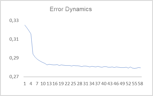
As you can see, in 10 epochs, the value of the root-mean-square error decreased to 0.28 and then continued to slowly decrease. It means, the autoencoder is able to compress information from 480 features (40 candles * 12 features per candle) up to a two-element latent state while preserving 78% of the information. If you remember, with PCA less than 25% of similar data is preserved on the first two components.

I deliberately use the latent state size equal to 2 elements. This enables its visualization and comparison to similar presentations we obtained using the Principal Component Analysis method. To prepare such data, let us slightly modify the above EA. The main changes will affect the model training function Train. The beginning of the function will not change — it includes the training sample creation process.

Right after creating the training sample, let us add training using the Principal Component Analysis method.

void Train(datetime StartTrainBar = 0)
  {
//---
    The process of creating a training sample has not changed
//---
   if(!PCA.Study(data))
     {
      printf("Runtime error %d", GetLastError());
      return;
     }

In the EA above, we created a system of two nested loops to train the model. Now we will not re-train the autoencoder, but we will use the previously trained model. Therefore, we do not need the system of nested loops. We only need one loop through the elements of the training sample. Also, we will not visualize the latent state for all 92,000 patterns. This will make the information hard to understand. I decided to visualize only 1000 patterns. You can repeat my experiments with any desired number of patterns for visualization.

Since I decided not to visualize the entire sample, I will randomly select a pattern for visualization from the training sample. So, we fill the temporary buffer with the features of the selected pattern.

     {
      //---
      stop = IsStopped();
      bool add_loop = false;
      for(int it = 0; i < 1000 && !stop; i++)
        {
         if((GetTickCount64() - last_tick) >= 250)
           {
            com = StringFormat("Calculation -> %d of %d -> %.2f%%", it + 1, 1000, (double)(it + 1.0) / 1000 * 100);
            Comment(com);
            last_tick = GetTickCount64();
           }
         int i = (int)((MathRand() * MathRand() / MathPow(32767, 2)) * (total));
         TempData.Clear();
         int r = i + (int)HistoryBars;
         if(r > bars)
            continue;
         //---
         for(int b = 0; b < (int)HistoryBars; b++)
           {
            int bar_t = r - b;
            double open = Rates[bar_t].open;
            TimeToStruct(Rates[bar_t].time, sTime);
            double rsi = RSI.Main(bar_t);
            double cci = CCI.Main(bar_t);
            double atr = ATR.Main(bar_t);
            double macd = MACD.Main(bar_t);
            double sign = MACD.Signal(bar_t);
            if(rsi == EMPTY_VALUE || cci == EMPTY_VALUE || atr == EMPTY_VALUE || macd == EMPTY_VALUE || sign == EMPTY_VALUE)
               continue;
            //---
            if(!TempData.Add(Rates[bar_t].close - open) || !TempData.Add(Rates[bar_t].high - open) ||
               !TempData.Add(Rates[bar_t].low - open) || !TempData.Add((double)Rates[bar_t].tick_volume / 1000.0) ||
               !TempData.Add(sTime.hour) || !TempData.Add(sTime.day_of_week) || !TempData.Add(sTime.mon) ||
               !TempData.Add(rsi) || !TempData.Add(cci) || !TempData.Add(atr) || !TempData.Add(macd) || !TempData.Add(sign))
               break;
           }
         if(TempData.Total() < (int)HistoryBars * 12)
            continue;

After receiving information about the pattern, call the autoencoder's feed forward method and compress the data using the Principal Component Analysis method. Then we get the value of the results buffer of the autoencoder's latent state.

         Net.feedForward(TempData, 12, true);
         data = PCA.ReduceM(TempData);
         TempData.Clear();
         if(!Net.GetLayerOutput(5, TempData))
            break;

Previously, when testing the models, we checked their ability to forecast the formation of a fractal. This time, to visually separate patterns, we will use color separation of patterns on the chart. Therefore, we need to specify which type the rendered pattern belongs to. To understand this, we need to check the formation of a fractal after the pattern.

         bool sell = (Rates[i - 1].high <= Rates[i].high && Rates[i + 1].high < Rates[i].high);
         bool buy = (Rates[i - 1].low >= Rates[i].low && Rates[i + 1].low > Rates[i].low);
         if(buy && sell)
            buy = sell = false;

The received data is saved to a file for further visualization. Then we move on to the next pattern.

         FileWrite(handle, (buy ? DoubleToString(TempData.At(0)) : " "), (buy ? DoubleToString(TempData.At(1)) : " "),
                   (sell ? DoubleToString(TempData.At(0)) : " "), (sell ? DoubleToString(TempData.At(1)) : " "),
                   (!(buy || sell) ? DoubleToString(TempData.At(0)) : " "),
                   (!(buy || sell) ? DoubleToString(TempData.At(1)) : " "),
                   (buy ? DoubleToString(data[0, 0]) : " "), (buy ? DoubleToString(data[0, 1]) : " "),
                   (sell ? DoubleToString(data[0, 0]) : " "), (sell ? DoubleToString(data[0, 1]) : " "),
                   (!(buy || sell) ? DoubleToString(data[0, 0]) : " "),
                   (!(buy || sell) ? DoubleToString(data[0, 1]) : " "));
         stop = IsStopped();
        }
     }

After all iterations of the loop, clear the comments field on the chart and close the EA.

   Comment("");
   ExpertRemove();
  }

The full EA code can be found in the attachment.

As a result of the Expert Advisor's operation, we have the AE_latent.csv file containing the data of the autoencoder's latent state and the first two principal components for the corresponding patterns. Two graphs were constructed using the data from the file.

Visualization of the latent state of an autoencoder Visualization of the 2 first principal components

As you can see, both presented graphs have no clear division of patterns into the desired groups. However, the autoencoder latency data is close to 0.5 on both axes. This time we used the sigmoid as an activation function for the neural layer of the latent state. And the function always returns a value in the range from 0 to 1. Thus, the center of the obtained distribution is close to the center of the range of function values.

Data compression using the Principal Component Analysis method gives quite large values. The values along the axes differ by 6-7 times. The center of the distribution is approximately at [18000, 130000]. There are also pronounced linear upper and lower limits of the range.

Based on the analysis of the presented graphs, I would choose an autoencoder for data pre-processing before the data is fed into the decision making neural network.

Conclusion

In this article, we got acquainted with autoencoders which are widely used to solve various problems. We built our first autoencoder using fully connected layers and compared its performance with Principal Component Analysis. The testing results showed the advantage of using an autoencoder when solving nonlinear problems. But the topic of Autoencoders is quite extensive and does not fit within one article. In the next article, I propose to consider various heuristics to improve the efficiency of autoencoders.

I will be happy to answer all your questions in the article's forum thread.

List of references

Programs used in the article

#	Name	Type	Description
1	ae.mq5	Expert Advisor	Autoencoder learning Expert Advisor
2	ae2.mq5	EA	EA for preparing data for visualization
2	NeuroNet.mqh	Class library	A library of classes for creating a neural network
3	NeuroNet.cl	Code Base	OpenCL program code library

Translated from Russian by MetaQuotes Ltd.
Original article: https://www.mql5.com/ru/articles/11172

Attached files |

Download ZIP

MQL5.zip (67.49 KB)

Warning: All rights to these materials are reserved by MetaQuotes Ltd. Copying or reprinting of these materials in whole or in part is prohibited.