Beyond the Clock (Part 1): Building Activity and Imbalance Bars in Python and MQL5

Table of Contents

1. Introduction
2. The Problem with Sampling on the Clock
3. Infrastructure: Parquet Storage and Dask Loading
4. Cleaning Tick Data Before Bar Construction
5. Standard Bars: Time, Tick, Volume, Dollar
6. Information Bars: Sampling on Market Intent
7. The Unified API — make_bars()
8. Bar Type Selection in Practice
9. MQL5 Implementation
10. Conclusion
11. Attached Files

Introduction

A model trained on one-minute bars inherits an assumption that has nothing to do with the market: that every 60-second window contains the same amount of information. It does not. A minute during the London open may carry hundreds of ticks and a directional move; a minute at 03:00 UTC on a Sunday may carry three ticks and zero signal. Treating both as equivalent observations injects heteroscedasticity at the data layer, before any feature is computed.

Chapter 1 of López de Prado's Advances in Financial Machine Learning replaces clock-based sampling with activity-based and intent-based alternatives. This article implements all ten bar types from that chapter in two implementations: a unified Python module (afml.data_structures.bars) for batch processing of multi-year tick histories, and an object-oriented MQL5 library for live tick-by-tick construction inside an Expert Advisor.

Four production problems in the pipeline are addressed explicitly: loading multi-year tick data without exceeding memory (partitioned Parquet storage read via Dask), cleaning broker-feed artifacts that corrupt bar construction (zero spreads, duplicate timestamps, NaT indices), calibrating the adaptive threshold for imbalance bars automatically so the first bar does not bias the EWM history, and persisting the EWM tracker across EA restarts so the threshold does not reset mid-session. A short parity test at the end verifies that the two implementations, fed the same tick stream, produce identical bars.

The Problem with Sampling on the Clock

Every ML pipeline for financial data begins with the same question: what is one observation? For most practitioners, the answer is a one-minute or five-minute OHLC bar — a fixed-time slice of the market. That choice is convenient and familiar, but it carries a structural flaw that propagates into every model trained on the resulting data.

Consider a liquid currency pair during the London open versus the same pair at 03:00 UTC on a Sunday. The former may generate hundreds of ticks per minute; the latter may generate fewer than five. A one-minute time bar treats these two samples as equivalent observations. The Sunday bar is almost entirely noise. The London bar is rich with information yet compressed to the same four numbers. As a result, we have a dataset with non-constant variance: the very condition that ARCH models were invented to describe, and one of the primary reasons financial returns are notoriously difficult to model with standard ML algorithms.

López de Prado formalizes this intuition in Chapter 1 of Advances in Financial Machine Learning (AFML). The core argument is that bars should close when a fixed amount of market activity has occurred, not when a fixed amount of time has elapsed. Activity can be measured in ticks, traded volume, or traded dollar value — each measure producing a different sampling scheme with different statistical properties. The most aggressive version of this idea, imbalance bars, closes a bar when the market's directional intent exceeds a threshold, capturing regime changes that none of the activity-based samplers can detect.

Bar construction is the upstream stage of any feature pipeline. The quality of downstream features — stationarity transforms, volatility estimates, and microstructural indicators — is bounded by the quality of the input bars. The Python implementation below resides in afml.data_structures.bars and exposes a single public function, make_bars(), covering all ten bar types discussed in AFML Chapter 1. The mirrored MQL5 implementation in §8 provides the same seven bar types in an event-driven form suitable for live trading inside an Expert Advisor, with additional infrastructure for state persistence across terminal disconnects.

Infrastructure: Parquet Storage and Dask Loading

The first lesson learned during implementation had nothing to do with sampling theory. Tick data for a single currency pair over a single calendar year can exceed 50 million rows. Loading that into a pandas DataFrame at session start takes minutes and consumes several gigabytes of RAM. Two changes eliminate both problems: store raw tick data in columnar Parquet format partitioned by year and month, and load it out-of-core using Dask rather than pandas.

The directory layout follows a simple convention:

tick_data_parquet/
  EURUSD/
    2023/
      month-01.parquet
      month-02.parquet
      ...
    2024/
      month-01.parquet
      ...

Each partition file is compressed with zstd via PyArrow. The compression ratio for floating-point tick data is typically 4:1 to 6:1 compared to raw CSV, and columnar storage means that loading only bid, ask, and volume columns skips the rest of the file entirely at the I/O layer.

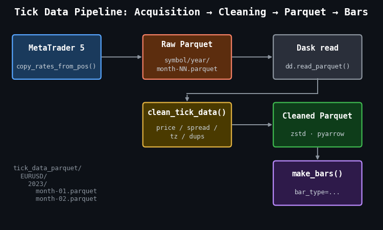
Figure 1: Single-pass illustration of the tick data pipeline from acquisition to bar construction

• MetaTrader 5: source of raw tick data via copy_rates_from_pos(), saved month-by-month into the raw Parquet tree.
• clean_tick_data(): validates prices, enforces positive spreads, localizes timestamps to UTC, removes duplicates, and sorts chronologically before writing to the cleaned store.
• Dask read: dd.read_parquet() with partition filters applies date predicates at the file level, so only the relevant month files are touched.
• make_bars(): receives a fully cleaned pandas DataFrame and dispatches to the appropriate bar constructor.

The load_tick_data() function wraps the Dask layer. It accepts a symbol, a date range, and an account name (used to verify that the loading environment matches the acquisition environment), applies row-group-level date filters, and calls .compute() to materialize the result as a pandas DataFrame for bar construction:

def load_tick_data(
    symbol: str,
    start_date,
    end_date,
    account_name: str,
    path=None,
    columns=None,
    verbose: bool = True,
) -> pd.DataFrame:
    root_path = Path(path) if path else Path.home() / "tick_data_parquet"
    if not verify_or_create_account_info(root_path, account_name):
        return pd.DataFrame()

    fname = root_path / symbol.upper()
    filters = [("time", ">=", start_date), ("time", "<=", end_date)]

    ddf = dd.read_parquet(fname, columns=columns, filters=filters, engine="pyarrow")
    return ddf.compute()

The practical consequence of this design becomes clear when querying a two-week window from a three-year dataset. Dask reads only the two or three monthly partition files that overlap the date range; the rest are skipped entirely. Without Parquet partitioning, the equivalent pandas workflow loads the entire dataset and then filters in memory — a pattern that fails entirely once the dataset exceeds available RAM.

Cleaning Tick Data Before Bar Construction

Bar construction produces wrong results if the input tick stream is not clean. The most common issues in MetaTrader 5 tick exports are negative or zero spreads (a known artifact of certain broker feed configurations), duplicate timestamps from reconnection events, and ticks arriving with NaT index entries when the MetaTrader 5 terminal loses connectivity.

The clean_tick_data() function applies seven sequential checks before the data reaches any bar constructor:

def clean_tick_data(
    df: pd.DataFrame,
    timezone: str = "UTC",
    min_spread: float = 1e-5,
) -> Optional[pd.DataFrame]:
    if df.empty:
        return None

    # 1. Ensure DatetimeIndex
    if not isinstance(df.index, pd.DatetimeIndex):
        df.index = pd.to_datetime(df.index)
        df = df[~df.index.isnull()]

    # 2. Timezone normalization
    df = df.tz_localize(timezone) if df.index.tz is None else df.tz_convert(timezone)

    # 3. Price validity: positive prices, ask > bid, spread >= min_spread
    price_filter = (
        (df["bid"] > 0)
        & (df["ask"] > 0)
        & (df["ask"] > df["bid"])
        & ((df["ask"] - df["bid"]) >= min_spread)
    )
    df = df[price_filter]

    # 4–7. Drop NaN, handle microseconds, remove duplicate timestamps, sort
    df.dropna(inplace=True)
    df = df[~df.index.duplicated(keep="last")]
    if not df.index.is_monotonic_increasing:
        df.sort_index(inplace=True)

    return df if not df.empty else None

One detail deserves attention: duplicates are resolved with keep="last" rather than keep="first". When a broker feed reconnects and resends the most recent tick, the resent version is more likely to have the corrected price. Keeping the last entry among duplicates matches that assumption.

Standard Bars: Time, Tick, Volume, Dollar

All four standard bar types share a single internal construction path. A grouper object partitions the tick DataFrame by bar membership; aggregation over each group produces OHLC prices, mean spread, and cumulative volume. The _make_bar_type_grouper() function encodes the partitioning logic for each type:

def _make_bar_type_grouper(
    df: pd.DataFrame,
    bar_type: str = "tick",
    bar_size: Union[int, str] = 100,
) -> tuple:
    if bar_type == "time":
        freq = set_resampling_freq(bar_size)
        return df.resample(freq, closed="left", label="right"), bar_size, None

    if bar_type == "tick":
        bar_id = np.arange(len(df)) // bar_size

    elif bar_type in ("volume", "dollar"):
        cum_metric = (
            df["volume"] * df["bid"] if bar_type == "dollar"
            else df["volume"]
        )
        bar_id = (cum_metric.cumsum() // bar_size).astype(int)

    return df.groupby(bar_id), bar_size, bar_id

Time Bars and the Zero-Tick-Volume Filter

Time bars are the only bar type where the grouper can produce empty groups. A one-hour bar during a market holiday or a session close contains zero ticks. That empty bar is not a data point — it is an absence of data — and passing it downstream propagates a silent error: the OHLC values for an empty group are undefined (pandas returns NaN), and the bar's tick_volume is zero, which causes division errors in any feature that normalizes by bar activity.

The production codebase introduced a zero-volume filter after observing this in practice. A batch of time bars constructed across a weekend gap contained 23 bars with tick_volume == 0. Those bars were populated with the previous close price carried forward by the resample aggregation, making them indistinguishable from real bars in the OHLC columns. The filter in _make_standard_bars() removes them and logs the count:

if bar_type == "time":
    eq_zero = ohlc_df["tick_volume"] == 0
    ohlc_df = ohlc_df[~eq_zero]

    nzeros = eq_zero.sum()
    if nzeros > 0:
        logger.info(
            f"Dropped {nzeros:,} of {ohlc_df.shape[0]:,} rows with zero tick volume."
        )

Figure 2: 2-panel illustration of the zero-tick-volume problem in time bars

• Panel (a): hourly tick density for a typical FX pair, with UTC hours 00–07 highlighted as the zero-tick risk zone. These hours correspond to late US session/Asian session close for majors.
• Panel (b): bar count before and after applying the zero-tick filter over a 5-day sample. 30 phantom bars are removed without affecting any tick that actually traded.

The filter does break the strict time sequencing of the bar index. A downstream component that assumes one bar per clock interval — for example, code that constructs a regular calendar join — will behave incorrectly after the filter. This is a deliberate tradeoff: a downstream model that receives phantom bars with carried-forward prices will produce worse predictions than one that receives a non-uniform but accurate time series.

Figure 3: 4-panel illustration of bar boundary placement for the four standard sampling methods

• Panel (a): time bars (blue), closing every 60 seconds. Boundaries are evenly spaced regardless of market activity.
• Panel (b): tick bars (green), closing every 100 ticks. Boundaries are also regular but aligned to activity count rather than clock time.
• Panel (c): volume bars (orange), closing when cumulative volume reaches a threshold. Boundaries cluster during high-volume periods and spread apart during quiet ones.
• Panel (d): dollar bars (purple), closing when cumulative dollar value reaches a threshold. Similar to volume bars but price-weighted, making the threshold more stable across symbols with different price scales.

Dollar Bars and Volatility Regime Sensitivity

The statistical argument for dollar bars over time bars is straightforward. A bar closes when a fixed dollar amount of the asset has changed hands. During active sessions, prices move more and volumes are higher, so the dollar threshold is reached quickly. During quiet sessions, the threshold takes longer to reach. The result is that each bar contains approximately the same amount of information regardless of the time it took to form.

This property produces return distributions that are closer to Gaussian than those from time bars, which matters because many ML algorithms (and virtually all risk models) assume independent, identically distributed returns. Figure 4 illustrates this on synthetic data with embedded volatility bursts.

Figure 4: 2-panel illustration of return distribution normality for time bars vs dollar bars

• Panel (a): time bar returns exhibit tail deviation from the normal reference line, particularly in the upper tail, reflecting the fat-tailed return distribution that arises when volatile and quiet periods are sampled at equal frequency.
• Panel (b): dollar bar returns track the normal reference line more closely across the full quantile range because each bar represents a fixed amount of traded value rather than a fixed amount of elapsed time.

Dollar bars are the recommended default for most ML applications in the pipeline. Tick bars are preferable when order flow is more informative than price times volume — for example, in markets where a single large order can be split into many small tickets. Volume bars sit between the two: they normalize for order size but not for price level, making them less stable across long backtesting windows where the asset price has drifted substantially.

Figure 5: 2-panel illustration of bar count sensitivity to volatility regimes

• Panel (a): time bars produce an identical count in calm and active regimes — the sampling clock does not respond to market conditions.
• Panel (b): dollar bars produce 5.6× more bars in the active regime than in the calm regime, concentrating observations precisely where market information is densest.

Information Bars: Sampling on Market Intent

Standard bars close on activity. Information bars close on directional activity — the net imbalance between buyer-initiated and seller-initiated trades. The idea is that a bar that closes when the market has committed to a direction contains more decision-relevant information than one that closes when a volume threshold is crossed regardless of direction.

The Tick Rule

Information bars require assigning a direction to each tick. The tick rule is the standard approach: a tick is classified as buyer-initiated (+1) if the price rose from the previous tick, seller-initiated (-1) if it fell, and inherits the previous classification if the price is unchanged:

@njit(cache=True)
def _tick_rule_kernel(prices: np.ndarray) -> np.ndarray:
    n = len(prices)
    b = np.empty(n, dtype=np.float64)
    b[0] = 1.0
    prev = 1.0

    for i in range(1, n):
        diff = prices[i] - prices[i - 1]
        if diff > 0.0:
            prev = 1.0
        elif diff < 0.0:
            prev = -1.0
        b[i] = prev

    return b

The @njit(cache=True) decorator compiles the loop to native machine code via Numba. The previous implementation used a pandas ffill() to propagate the last non-zero sign forward; replacing it with an explicit carry-forward variable inside a Numba kernel eliminates the pandas overhead entirely. On 500,000 ticks the compiled version completes in less than 1 ms.

The direction array b is stored as float64 rather than int8. That choice is intentional: the values {−1.0, +1.0} are immediately multiplied against floating-point metrics (volume, price, dollar value) inside the same kernel. Storing them as float64 eliminates a cast on every multiply. The alternative — allocating b as int8 to save eight bytes per tick — saves 500 KB on a million-tick dataset while adding a cast instruction on every multiply-add in the boundary loop. The Numba JIT generates identical machine code for both variants once the cast is present; the float64 layout simply skips it.

The tick rule is a proxy. It misclassifies a meaningful fraction of trades, particularly in markets where the bid-ask spread is wide relative to the tick size. The Lee-Ready algorithm improves classification accuracy for datasets that include the quoted bid and ask at each trade, but the tick rule is sufficient for the purposes of imbalance bar construction and avoids the additional complexity of mid-quote comparisons.

Imbalance Bars

A tick imbalance bar closes when the cumulative signed metric θT exceeds a threshold derived from the expected bar length and the expected per-tick imbalance. For tick imbalance bars, the metric per tick is simply bt. For volume imbalance bars, it is bt · vt. For dollar imbalance bars, it is bt · pt · vt. The bar closes at tick T when:

|θT| ≥ E0[T] · |E0[imbalance per tick]|

Both expectations on the right-hand side are updated after each completed bar using an exponentially weighted mean (EWM). The EWM span controls how quickly the threshold adapts to a new regime. A short span (5–10 bars) produces an aggressive tracker that may generate very small bars during a trend; a long span (50–100 bars) produces a stable threshold that responds slowly to regime changes. The caller converts the span to a decay factor α = 2 / (span + 1) before entering the loop.

The critical implementation detail is how the EWM is computed. The original implementation kept two growing Python lists and rebuilt a pd.Series at each bar close to compute .ewm().mean().iloc[-1]. That approach is O(n) per call and O(n²) total across all bars — at 500,000 ticks it consumed 92% of the boundary detection runtime. The adjust=False EWM is a one-line recurrence: ewm = α·x + (1−α)·ewm. Inlining that recurrence as two scalar updates inside a Numba JIT loop reduces the per-bar cost to O(1) and the total boundary detection time by over 1,000×.

The implementation in _detect_imbalance_boundaries() maintains two incremental EWM scalars — one for the expected bar length, one for the expected absolute imbalance — updated with a single multiply-add at each bar close:

@njit(cache=True)
def _detect_imbalance_boundaries(
    metric: np.ndarray,
    exp_ticks_init: float,
    exp_imbalance_init: float,
    ewm_alpha: float,
) -> np.ndarray:
    n = len(metric)
    boundaries = np.empty(n, dtype=np.int64)
    n_bars = 0

    theta = 0.0
    bar_start = 0

    # Incremental EWM state (O(1) per bar close)
    ewm_T = exp_ticks_init
    ewm_abs_theta = abs(exp_imbalance_init) * exp_ticks_init
    exp_T = exp_ticks_init
    exp_abs_imb = abs(exp_imbalance_init)
    one_minus_alpha = 1.0 - ewm_alpha

    for t in range(n):
        theta += metric[t]
        threshold = exp_T * exp_abs_imb

        if abs(theta) >= threshold:
            boundaries[n_bars] = t
            n_bars += 1

            bar_len = float(t - bar_start + 1)

            # O(1) EWM update: ewm = α·x + (1-α)·ewm
            ewm_T = ewm_alpha * bar_len + one_minus_alpha * ewm_T
            ewm_abs_theta = ewm_alpha * abs(theta) + one_minus_alpha * ewm_abs_theta

            exp_T = ewm_T
            exp_abs_imb = ewm_abs_theta / max(exp_T, 1.0)

            theta = 0.0
            bar_start = t + 1

    return boundaries[:n_bars]

Figure 6: 3-panel illustration of tick imbalance bar construction on a synthetic tick stream

• Panel (a): per-tick direction signal bt ∈ {+1, −1} from the tick rule. Yellow vertical lines mark bar boundaries.
• Panel (b): cumulative imbalance θT (green) with adaptive ±threshold bands (orange dashed). A bar closes each time θT touches or crosses a band; the threshold narrows or widens as the EWM updates.
• Panel (c): mid price with bar boundaries. This stream of 800 ticks produces 10 imbalance bars — significantly fewer than the 8–16 bars that fixed-size samplers would produce from the same input.

Automatic Threshold Calibration

AFML presents the imbalance bar recurrence relation clearly. What it does not discuss is the initialization problem that every production implementation must solve: what are the correct values for E0[T] and E0[imbalance per tick] at bar zero?

The choice of E0[T] determines the threshold for the very first bar. If E0[T] is set too low — say, 10 ticks — the first bar closes almost immediately, producing a poor seed for the EWM history. The subsequent adaptation is then anchored to that poor seed for many bars before recovering. If E0[T] is set too high — say, 10,000 ticks — the first bar never closes during a short backtesting window, returning an empty DataFrame with no error and no warning.

The updated implementation solves this automatically. Passing target_timeframe to make_bars() calls _calibrate_information_bar_params() internally, which derives both initial values from the tick data itself. target_timeframe is an MetaTrader 5 timeframe string that expresses the desired bar cadence — 'M5', 'M15', 'H1', and so on. The calibrator computes the median tick count per period at that timeframe for E0[T], and estimates the empirical directional bias |E[bt]| from up to 500,000 ticks for E0[imbalance per tick], floored at 0.01 so the threshold does not collapse to zero on a perfectly symmetric tape:

# Preferred — auto-calibrated dollar imbalance bars targeting M15 cadence
dimb_bars = make_bars(tick_df, bar_type="dollar_imbalance", target_timeframe="M15")

# Advanced — explicit initialization when calibration has been done offline
dimb_bars = make_bars(
    tick_df,
    bar_type="dollar_imbalance",
    exp_ticks_init=11_700,
    exp_imbalance_init=0.02,
)

The two forms are mutually exclusive: passing target_timeframe together with exp_ticks_init or exp_imbalance_init raises ValueError. Passing neither for an information bar type also raises ValueError, with a message that names the missing parameter and gives an example. Standard bar types are unaffected — target_timeframe is silently ignored for 'tick', 'time', 'volume', and 'dollar'.

For volume and dollar imbalance bars, the calibrator scales the imbalance estimate by the mean tick volume or mean dollar value respectively, so the threshold has the correct units. The result is that a single target_timeframe='M15' call produces bars that close at roughly the same cadence regardless of whether the metric is a direction, a volume, or a dollar value.

The practical recommendation for live trading: compute the calibration once offline using the full tick history, store the resulting exp_ticks_init and exp_imbalance_init in a JSON configuration file, and pass them explicitly to the MQL5 EA at startup. The auto-calibration pass in Python sees the full multi-year dataset; the equivalent step in MQL5 is constrained to whatever tick history the terminal has cached locally, which may be as little as the last week.

The Unified API — make_bars()

All ten bar types are accessible through a single entry point. The function validates the bar type, computes derived columns (mid price, spread, spread in basis points) shared by all types, dispatches to the appropriate internal constructor, and applies shared post-processing (timezone stripping, dtype downcasting, logging):

from afml.data_structures.bars import make_bars

# Standard bars — unchanged interface
time_bars   = make_bars(tick_df, bar_type="time",   bar_size="M5")
tick_bars   = make_bars(tick_df, bar_type="tick",   bar_size=500)
vol_bars    = make_bars(tick_df, bar_type="volume", bar_size=100_000)
dollar_bars = make_bars(tick_df, bar_type="dollar", bar_size=10_000_000)

# Information bars — preferred: let the function derive both initial values
timb_bars = make_bars(tick_df, bar_type="tick_imbalance",   target_timeframe="M15")
vimb_bars = make_bars(tick_df, bar_type="volume_imbalance", target_timeframe="M15")
dimb_bars = make_bars(tick_df, bar_type="dollar_imbalance", target_timeframe="M15")

# Information bars — advanced: explicit initialization skips auto-calibration
dimb_bars = make_bars(
    tick_df,
    bar_type="dollar_imbalance",
    exp_ticks_init=300,
    exp_imbalance_init=0.08,
)

Every call returns a DataFrame indexed by bar-close time with consistent column names:

Column	Type	Notes
open, high, low, close	float32	OHLC prices; mid_price by default
spread	float32	Mean bid-ask spread over the bar
spread_bps	float32	Spread in basis points
tick_volume	int32	Number of ticks in the bar
volume	float32	Sum of traded volume; present when source data includes volume
tick_num	int64	1-based global tick index at bar close; enables event-driven joins

The tick_num column deserves a note. When the bar DataFrame is joined to the original tick stream for event-driven labeling (the triple-barrier method, for example), the join key must be the tick index rather than the timestamp. Two bars that close within the same microsecond — which can happen for very small imbalance bars during news events — have identical timestamps but distinct tick indices. The tick_num column makes that join unambiguous.

Bar Type Selection in Practice

No single bar type dominates across all instruments and all pipeline stages. The following heuristics reflect what emerged from building the full pipeline rather than from the theoretical arguments alone.

Condition	Recommended type
General-purpose default, liquid FX or equity	Dollar bars
Order-flow studies, fragmented execution markets	Tick bars
Commodity or futures with stable lot sizes	Volume bars
Regime detection, directional signal validation	Tick or dollar imbalance bars
Baseline comparison, human-readable reporting	Time bars (with zero-tick filter)

Imbalance bars are not universally better. They produce variable-length bars that complicate fixed-window feature engineering, and their bar count is sensitive to ewm_span in ways that are difficult to reason about without running the full construction pass. The target_timeframe parameter mitigates this by anchoring the initial threshold to a familiar cadence, but the realized count still fluctuates with volatility and volume. For a first modeling iteration, dollar bars with a threshold calibrated to produce 30–50 bars per trading session are a stable and reproducible choice. Imbalance bars become valuable once the standard bar pipeline is validated and the downstream model is known to benefit from regime-adaptive sampling.

MQL5 Implementation

The Python module above consumes ticks in batch: a fully materialized DataFrame is partitioned by bar membership, aggregated, and returned in one pass. An MQL5 Expert Advisor consumes ticks one at a time in OnTick(), with no look-ahead, no vectorization, and three burdens the Python side gets for free: gap handling when the terminal disconnects, persistence of the imbalance-bar EWM state across EA restarts, and warm-up of the tick rule when the EA attaches mid-stream. These are complementary implementations of the same specification. Production parity requires handling each of these constraints explicitly.

The MQL5 implementation lives in three header files and one example Expert Advisor:

• CBarConstructor.mqh: abstract base class that owns the OHLC accumulator, the bar-emission struct, and the state-persistence interface.
• CStandardBars.mqh: concrete classes CTimeBar, CTickBar, CVolumeBar, and CDollarBar, mirroring the Python standard bar types.
• CImbalanceBars.mqh: CTickRule tick-direction classifier and CImbalanceBar constructor with the EWM threshold state, covering tick, volume, and dollar imbalance variants.
• BarBuilderEA.mq5: example EA that instantiates the selected bar type, processes live ticks, appends closed bars to CSV, and serializes state via OnInit()/OnDeinit().

Class Hierarchy

A single polymorphic base class factors out the shared bar state — OHLC accumulator, tick and volume counters, spread tracker, emission struct — and exposes one pure virtual method, ProcessTick(), that each derived class implements according to its own close semantics. The design reflects a subtle asymmetry in the López de Prado specification: the boundary tick — the tick that triggers bar closure — belongs to different bars for different bar types.

• Tick bars: close when m_tick_volume == bar_size. The (bar_size + 1)-th tick is the first of the new bar.
• Volume and dollar bars: close when a global cumulative metric crosses a multiple of bar_size. The crossing tick is the first of the new bar, consistent with Python's cumsum // bar_size semantics.
• Imbalance bars: close when |θ| ≥ threshold after the latest tick is added. The crossing tick is the last of the closing bar, consistent with Python's boundaries[n_bars] = t convention in _detect_imbalance_boundaries().

Conflating the three would produce a bar sequence that differs from the Python reference by one tick at every boundary — a drift that accumulates over long backtests and breaks parity entirely for imbalance bars. The MQL5 class hierarchy honors each semantic explicitly.

Figure 7. Three-level inheritance diagram of the MQL5 bar-constructor classes

• Level 1: CBarConstructor (abstract) owns the shared OHLC accumulator and exposes the pure-virtual ProcessTick() plus the SaveState / LoadState persistence interface.
• Level 2: four direct children implement the close semantics — CTimeBar, CTickBar, the intermediate abstract CCumSumBar, and CImbalanceBar. The orange border on CImbalanceBar marks the only class with additional persisted state beyond the base accumulator.
• Level 3: CVolumeBar and CDollarBar derive from CCumSumBar, differing only in the per-tick metric returned by TickMetric().

The base class declares the shared state and three non-virtual helpers — SeedBar(), UpdateAccumulator(), and FillBar() — that every derived class calls in a different order:

//+------------------------------------------------------------------+
//| Emitted bar record. Fields mirror the columns produced by the    |
//| Python make_bars() function exactly.                             |
//+------------------------------------------------------------------+
struct SBar
  {
   datetime          time;           // Bar close time (right edge for time bars,
   // last-tick time for all other bar types)
   double            open;           // Open price (bid of the first tick in bar)
   double            high;           // High price (max bid observed in bar)
   double            low;            // Low price  (min bid observed in bar)
   double            close;          // Close price (bid of the last tick in bar)
   double            mid_open;       // Mid-price at bar open
   double            mid_close;      // Mid-price at bar close
   long              tick_volume;    // Number of ticks in the bar
   double            volume;         // Sum of tick.volume (tick-volume proxy on FX)
   double            spread;         // Mean (ask - bid) over the bar
   long              tick_num;       // 1-based global tick index at bar close
   string            bar_type;       // "time" | "tick" | "volume" | "dollar"
   //  | "tick_imbalance" | "volume_imbalance"
   //  | "dollar_imbalance"
  };

//+------------------------------------------------------------------+
//| Abstract base class. Owns the OHLC accumulator and emission      |
//| plumbing. Each derived class implements ProcessTick() with the   |
//| close semantics for its bar type.                                |
//+------------------------------------------------------------------+
class CBarConstructor
  {
protected:
   //--- Bar accumulator state
   bool              m_initialized;
   double            m_open, m_high, m_low, m_close;
   double            m_mid_open, m_mid_close;
   long              m_tick_volume;
   double            m_volume;
   double            m_spread_sum;
   datetime          m_last_tick_time;
   long              m_last_tick_num;
   long              m_bar_start_tick_num;
   string            m_bar_type;

   //--- Seed the accumulator with the first tick of a new bar
   void              SeedBar(const MqlTick &tick, const long tick_num);

   //--- Fold a subsequent tick into the running OHLC/volume/spread
   void              UpdateAccumulator(const MqlTick &tick, const long tick_num);

   //--- Copy closed-bar state into the caller's SBar
   void              FillBar(SBar &bar);

public:
                     CBarConstructor(const string bar_type);
   virtual          ~CBarConstructor(void) {}

   //--- Feed one tick. Returns true iff a bar closed on this call.
   //--- When true, the closed bar is written into out_bar by reference.
   virtual bool      ProcessTick(const MqlTick &tick,
                                 const long tick_num,
                                 SBar &out_bar) = 0;

   //--- State persistence for EA restart recovery. Derived classes
   //--- with additional state (e.g. CImbalanceBar) override to chain.
   virtual bool      SaveState(const int file_handle);
   virtual bool      LoadState(const int file_handle);

   //--- Accessors
   string            BarType(void) const { return m_bar_type; }
   bool              IsInitialized(void) const { return m_initialized; }
  };

SeedBar() initializes the OHLC accumulator from the first tick of a new bar, UpdateAccumulator() folds a subsequent tick into the running OHLC/volume/spread statistics, and FillBar() copies the closed-bar state into the caller's SBar. The derived classes differ only in which order they call these helpers relative to the close-decision check.

The simplest derived class is CTickBar, which closes when the tick count reaches bar_size:

//+------------------------------------------------------------------+
//| CTickBar — closes when tick count in the current bar reaches     |
//| bar_size. The (bar_size+1)-th tick is the first of the new bar,  |
//| matching Python's np.arange(len(df)) // bar_size semantics.      |
//+------------------------------------------------------------------+
class CTickBar : public CBarConstructor
  {
private:
   int               m_bar_size;

public:
                     CTickBar(const int bar_size) : CBarConstructor("tick")
     {
      m_bar_size = bar_size;
     }

   virtual bool      ProcessTick(const MqlTick &tick,
                            const long tick_num,
                            SBar &out_bar) override
     {
      if(!m_initialized)
        {
         SeedBar(tick, tick_num);
         return false;
        }

      if(m_tick_volume >= m_bar_size)
        {
         FillBar(out_bar);
         SeedBar(tick, tick_num);
         return true;
        }

      UpdateAccumulator(tick, tick_num);
      return false;
     }
  };

Volume and dollar bars share an intermediate parent class CCumSumBar that maintains a global cumulative metric and a bar identifier derived from its floor division by bar_size. Derived classes differ only in the per-tick metric — tick.volume for CVolumeBar, tick.bid * tick.volume for CDollarBar — exposed through a pure-virtual TickMetric() method. The imbalance-bar constructor follows the same three-helper pattern but adds the tick rule and the O(1) EWM recurrence, which are covered in §8.3.

OnTick Integration and CSV Output

The EA holds a single CBarConstructor* instance, instantiated in OnInit() according to an input parameter, and calls its ProcessTick() method on every incoming tick. The SBar is passed by reference to ProcessTick(), so no heap allocation occurs per bar close. When ProcessTick() returns true, the EA appends the closed bar to the output CSV.

The CSV output uses append semantics rather than overwrite. OpenCsvOutput() checks whether the output file already exists before opening it. If the file is new or empty, a header row is written; if the file exists and is non-empty, the file pointer is moved to the end and bar rows accumulate without truncating prior session data. This is the correct behavior for a live EA that may restart dozens of times across a multi-day session:

//+------------------------------------------------------------------+
//| CSV output helpers (using dynamic file name)                     |
//+------------------------------------------------------------------+
bool OpenCsvOutput(void)
  {
//--- Open in append mode if the file exists; else create with header
   bool existed = FileIsExist(g_outputFile);
   g_csv_handle = FileOpen(g_outputFile,
                           FILE_WRITE | FILE_READ | FILE_CSV | FILE_ANSI,
                           ',');
   if(g_csv_handle == INVALID_HANDLE)
     {
      PrintFormat("OpenCsvOutput: FileOpen('%s') failed, err=%d",
                  g_outputFile, GetLastError());
      return false;
     }

   FileSeek(g_csv_handle, 0, SEEK_END);
   if(!existed || FileTell(g_csv_handle) == 0)
     {
      FileWrite(g_csv_handle,
                "time", "open", "high", "low", "close",
                "mid_open", "mid_close",
                "tick_volume", "volume", "spread",
                "tick_num", "bar_type");
     }
   return true;
  }

The output CSV now also includes mid_open and mid_close, matching the additional mid-price fields added to SBar in this revision. The parity test in §8.4 aligns on tick_num, which is unaffected by the header change.

State Persistence with Staleness Detection

State persistence matters only for imbalance bars, and only in the live setting. When the terminal disconnects and reconnects, the EA is re-initialized; if the EWM scalars reset to their exp_ticks_init and exp_imbalance_init seeds, the threshold reverts to its bar-zero value. The bar that closes immediately after the restart will be sized using stale expectations, and several subsequent bars will be contaminated before the EWM re-converges.

The fix is to serialize the EWM state in OnDeinit() and deserialize it in OnInit(). First, the timestamp of the save is written at the head of the state file; RestoreState() reads it before loading any bar data and discards the file if the gap exceeds InpStateMaxAgeMin. Second, OnDeinit() deletes the state file when the EA is removed by the user (reason == REASON_REMOVE) so a stale file from an abandoned chart does not contaminate a fresh deployment on the same symbol:

//+------------------------------------------------------------------+
//| State file helpers (using dynamic file name)                     |
//+------------------------------------------------------------------+
bool RestoreState(void)
  {
   if(!InpUseStateFile)
      return false;
   if(!FileIsExist(g_stateFile, FILE_COMMON))
      return false;

   int fh = FileOpen(g_stateFile, FILE_READ | FILE_BIN | FILE_COMMON);
   if(fh == INVALID_HANDLE)
     {
      PrintFormat("RestoreState: FileOpen(%s) failed, err=%d", g_stateFile, GetLastError());
      return false;
     }

//--- Check staleness
   datetime saved = (datetime)FileReadLong(fh);
   if((TimeCurrent() - saved) > (InpStateMaxAgeMin * 60))
     {
      FileClose(fh);
      PrintFormat("State file %s is stale (saved at %s); discarding.",
                  g_stateFile, TimeToString(saved));
      return false;
     }

   g_tick_num = FileReadLong(fh);
   bool ok = g_bar.LoadState(fh);
   FileClose(fh);

   if(ok)
      PrintFormat("State restored from %s: saved=%s, tick_num=%d, type=%s",
                  g_stateFile, TimeToString(saved), g_tick_num, g_bar.BarType());
   return ok;
  }

FILE_COMMON is used so the state file is shared across all terminals running the EA — relevant when a portfolio of charts uses the same symbol and one terminal disconnects while another continues. The SaveState()/LoadState() methods in the base class persist the OHLC accumulator and tick counters. CImbalanceBar overrides both to chain the base implementation and then write/read its additional EWM scalars: m_theta, m_ewm_T, m_ewm_abs_theta, m_exp_T, m_exp_abs_imb, m_bar_tick_count, and the tick rule's prev_price and prev_sign.

Initialization: Supplying exp_ticks_init to the EA

The MQL5 EA still receives InpExpTicksInit and InpExpImbInit as explicit input parameters rather than computing them automatically. This is a deliberate constraint, not an oversight. The Python _calibrate_information_bar_params() function scans up to 500,000 ticks and runs the full tick-rule kernel before the first bar is constructed. MQL5's CopyTicksRange() is constrained by whatever the terminal has cached locally, which may be as little as the last week and is guaranteed to miss weekend gaps, low-volume holidays, and overnight sessions — exactly the samples that anchor E0[T] correctly. Performing auto-calibration inside OnInit() from a shallow history would produce a threshold that is biased toward the most recent market conditions, which is the opposite of what a stable initializer should do.

The recommended workflow is to run Python auto-calibration offline against the full multi-year Parquet dataset, write the result to a JSON configuration file in MQL5\Files\Common, and read it in OnInit():

# Python: one-time offline calibration against full tick history
bars = make_bars(tick_df, bar_type="dollar_imbalance", target_timeframe="M15")
# Retrieve the seeds that were used internally
config = {"exp_ticks_init": bars.attrs["exp_ticks_init"],
          "exp_imbalance_init": bars.attrs["exp_imbalance_init"]}
with open("EURUSD_imbalance_config.json", "w") as f:
   json.dump(config, f)

The MQL5 side reads this file in OnInit() and passes the values directly to CImbalanceBar. If the config file is absent, the EA falls back to InpExpTicksInit and InpExpImbInit — the user-supplied inputs — with a logged warning. A fallback that uses CopyTicksRange() over the recent local history is available in the attached source but is not recommended for the reasons above.

Parity Verification Against the Python Baseline

The two implementations target the same specification. If they disagree, one of them has a bug — and it is much easier to find which by comparing bars than by reading code. The verification procedure is straightforward: run the EA in the Strategy Tester over a defined historical tick window with Every tick based on real ticks mode, export the bars to CSV via FILE_COMMON, load both the CSV and the Python make_bars() output in a notebook, and align them by tick_num.

import pandas as pd
from afml.data_structures.bars import make_bars
from afml.mt5.clean_data import clean_tick_data

tick_df = pd.read_parquet("EURUSD_2024_01_15.parquet")
tick_df = clean_tick_data(tick_df)

py_bars  = make_bars(tick_df, bar_type="dollar", bar_size=10_000_000)
mql_bars = pd.read_csv("bars_dollar.csv", parse_dates=["time"])

merged = py_bars.merge(mql_bars, on="tick_num",
                       suffixes=("_py", "_mql"), how="outer", indicator=True)

for col in ["open", "high", "low", "close", "tick_volume"]:
   diff = (merged[f"{col}_py"] - merged[f"{col}_mql"]).abs()
   assert diff.max() < 1e-8, f"Mismatch in {col}: max diff {diff.max()}"

print(f"Parity verified across {len(merged)} bars")

Figure 8. Two-panel parity verification on a 1,200-tick synthetic slice with three embedded volatility regimes

• Panel (a): bid price (grey) with dollar-bar close boundaries from Python (blue, wider) and MQL5 (orange, dashed) drawn on top. Exact agreement shows as orange dashes sitting inside every blue band.
• Panel (b): per-bar absolute difference in tick_num between the two implementations. All 25 bars register zero difference, annotated in the top-right corner. Any non-zero bar indicates a divergence that must be resolved before deployment.

The three most common parity failures in practice are an off-by-one at the first bar (the EA sees a bid-only tick that Python's clean_tick_data() rejects for negative spread), systematic drift in dollar bars (the two sides use different prices for the dollar metric), and diverging EWM after a restart (the MQL5 run starts fresh while the Python run sees the full stream). The CSV append logic introduced in §8.2 does not affect parity: the bar values written per session are identical to a single-session run; only the file structure changes. When running the parity test, point the Python comparison at the same day's rows by filtering on time before the merge.

Conclusion

Time bars are the default because they are easy to construct, not because they are correct. Every assumption that makes financial ML harder — non-constant variance, serial correlation, overrepresentation of quiet periods — traces in part to the fixed-clock sampling convention. The bar types in afml.data_structures.bars replace that convention with one grounded in market activity: dollar value, tick count, traded volume, or directional imbalance.

Four implementation details separate a working bar constructor from one that produces subtly wrong training data. The first is the zero-tick-volume filter for time bars: phantom bars from market closures and holidays look identical to real bars in the OHLC columns and must be explicitly removed. The second is automatic threshold calibration for imbalance bars: passing target_timeframe to make_bars() now derives E0[T] and E0[imbalance per tick] internally from the tick data, eliminating the manual warm-up pass that AFML leaves implicit. The third is unique to live deployment: the EWM state of imbalance bars must be persisted across EA restarts, with a staleness check so that a quiet Friday close does not set an inappropriate threshold for a Monday news open. The fourth is CSV append semantics in the EA: opening the output file in overwrite mode silently discards all bars produced before the last restart, which defeats the purpose of per-session logging.

The infrastructure layer — partitioned Parquet storage read via Dask — is not optional for anything beyond a small toy dataset. A single year of tick data for a single currency pair exceeds what most workstations can hold in memory, and the penalty for loading more than is needed grows with dataset size. Partitioning by year and month, combined with Dask's row-group-level date filters, keeps memory usage bounded regardless of the backtesting window requested.

Attached Files

Copy the AlternativeBars folder to MQL5/Include/ and BarBuilderEA.mq5 to MQL5/Experts/ before compiling.

File	Description
MQL5
AlternativeBars\CBarConstructor.mqh	Abstract base class: shared OHLC accumulator, SBar emission struct (including mid_open and mid_close), and SaveState/LoadState persistence interface
AlternativeBars\CStandardBars.mqh	CTimeBar, CTickBar, CCumSumBar, CVolumeBar, and CDollarBar — the four standard bar types
AlternativeBars\CImbalanceBars.mqh	CTickRule direction classifier and CImbalanceBar with ENUM_IMBALANCE_METRIC selector (tick, volume, dollar), EWM-adaptive threshold, diagnostic accessors (CurrentTheta, CurrentThreshold, ExpT, ExpAbsImb), and full state persistence
BarBuilderEA.mq5	Example Expert Advisor: factory instantiation for seven bar types, append-mode CSV output with header detection, staleness-aware state restore in OnInit(), and state-file deletion on REASON_REMOVE in OnDeinit()
Python — afml/data_structures/
afml/data_structures/bars.py	Unified make_bars() entry point: target_timeframe as the primary interface for information bars (auto-calibrates both initial EWM seeds from the data); exp_ticks_init / exp_imbalance_init retained as mutually exclusive escape hatches for advanced use
afml/data_structures/information_bars.py	JIT-compiled boundary detection for all six information bar types; tick-rule kernel, O(1) EWM recurrence in _detect_imbalance_boundaries(), and vectorized aggregation via np.add.reduceat
afml/data_structures/calibration.py	_calibrate_information_bar_params(): derives E0[T] from median tick density at the target timeframe, and E0[imbalance per tick] from the empirical directional bias over up to 500,000 ticks, scaled to the correct units for volume and dollar variants