
Neural Networks in Trading: Dual Clustering of Multivariate Time Series (Final Part)

Introduction
We continue working on implementing the approaches proposed by the authors of the DUET framework for dual clustering of multivariate time series, which represents a powerful tool for financial market forecasting. DUET combines temporal and channel clustering, enabling adaptation to complex and evolving patterns of market dynamics while overcoming the limitations of traditional methods prone to overfitting and limited flexibility.
DUET includes several key modules, each performing a critically important role. The first stage of data processing involves normalization and outlier removal, which improves model robustness.
This is followed by temporal clustering, which partitions the time series into groups with similar dynamics. This allows the model to account for phase shifts in market processes, which is especially important when analyzing highly volatile assets.
Channel clustering is used to identify the most significant variables among numerous market factors. Financial data contains a substantial amount of noise and redundant information, which hinders accurate forecasting. DUET analyzes correlations between parameters and eliminates insignificant components, concentrating computational resources on key features. Frequency-domain signal analysis and latent feature extraction mechanisms make the model less sensitive to random market fluctuations.
The data fusion module synchronizes information obtained from the temporal and channel clustering modules, forming a unified representation of the analyzed environmental state. This stage is based on a masked attention mechanism that enables the model to focus on the most relevant characteristics while minimizing the influence of unrepresentative data. As a result, DUET demonstrates high robustness to dynamic changes and improves long-term forecasting performance.
The final forecasting module uses aggregated features to compute future values of time series. This stage relies on advanced neural network methods capable of capturing nonlinear dependencies between market indicators. The flexibility of the DUET architecture allows it to dynamically adapt to various conditions, eliminating the need for manual parameter tuning.
An original visualization of the DUET framework is provided below.

In the practical section of the previous article, we presented an implementation of the temporal clustering module. We continue this work and proceed to the construction of the channel clustering module.
Channel Clustering Module
The channel clustering module addresses the problem of properly accounting for inter-channel relationships when forecasting multivariate time series. Here, the authors of the DUET framework employ metric learning aimed at clustering channels in the frequency domain.
A key aspect of CCM is the representation of data in the frequency domain. To achieve this, time series are decomposed into frequency components using the Fast Fourier Transform (FFT). As a result, signals are analyzed in the spectral domain, where inter-channel relationships become more explicit. Many hidden dependencies that are not visible in traditional analysis emerge only after transformation into the frequency domain, making this approach particularly valuable for complex time series.
Inter-channel relationships are evaluated using a learnable distance metric. The amplitude representation of the frequency spectrum is used as the base measure, and the distance is computed using a modified Mahalanobis metric. This method accounts not only for pairwise distances between channels but also for their correlations in spectral space.
After computing distances between channels, a relationship matrix is formed, with coefficients normalized to the range [0, 1]. This normalization enables the identification of the most significant connections while eliminating weak and noisy fluctuations.
For final information filtering, a binary channel masking matrix is constructed. This process is based on probabilistic sampling, where each channel is assigned a probability of usefulness for forecasting. Such a mechanism allows uncertainty in the data to be taken into account and avoids rigid thresholding. As a result, the model automatically excludes insignificant channels, significantly improving interpretability and reducing information redundancy.
Within the scope of this work, we implement a slightly simplified version of the channel clustering module. The discrete Fourier transform algorithm was previously implemented as part of the FITS framework and is already available in our library. Instead of the Mahalanobis metric, a simpler method based on vector distances between frequency amplitude components is used. This preserves the advantages of frequency analysis while reducing computational complexity and simplifying the algorithm.
After transforming time series into the frequency domain, the norms of the amplitude spectra for each channel are computed. Then, pairwise distances are calculated to form an inter-channel relationship matrix. To eliminate weak dependencies from further analysis, normalization is applied, suppressing noise and scaling distances. Thus, only significant correlations between channels are retained. Based on this matrix, a probabilistic model of relationships is constructed. Each channel is assigned a significance weight reflecting its influence on other series.
The described algorithm is implemented in the MaskByDistance kernel on the OpenCL side. The kernel parameters include pointers to three data buffers. The first two contain the input data in the form of real and imaginary parts of the analyzed signals, while the third is used to store the results. In this case, it contains the channel masking matrix.
__kernel void MaskByDistance(__global const float *buf_real,
                             __global const float *buf_imag,
                             __global float *mask,
                             const int dimension
                            )
  {
   const size_t main = get_global_id(0);
   const size_t slave = get_local_id(1);
   const int total = (int)get_local_size(1);
Within the kernel body, the current thread is first identified in a two-dimensional execution space. The first dimension corresponds to the analyzed channel, and the second to the channel being compared. Workgroups are formed along the second dimension.
Next, a local memory array is created for data exchange between threads within the same workgroup.
__local float Temp[LOCAL_ARRAY_SIZE];
int ls = min((int)total, (int)LOCAL_ARRAY_SIZE);
Offsets in the global data buffers are then determined.
const int shift_main = main * dimension;
const int shift_slave = slave * dimension;
const int shift_mask = main * total + slave;
After the preparatory steps, computation begins with a loop that calculates the distance between two vectors of frequency amplitudes.
//--- calc distance
   float dist = 0;
   if(main != slave)
     {
#pragma unroll
      for(int d = 0; d < dimension; d++)
         dist += pow(ComplexAbs((float2)(buf_real[shift_main + d], buf_imag[shift_main + d])) -
                     ComplexAbs((float2)(buf_real[shift_slave + d], buf_imag[shift_slave + d])), 2.0f);
      dist = sqrt(dist);
     }
Note that diagonal elements exist in the thread matrix. As expected, in such cases the algorithm computes the distance between two identical vectors, which is obviously equal to zero. Therefore, the distance computation loop is skipped, and a zero value is directly assigned.
Next, we need to normalize the values. For this purpose, let us implement an algorithm to find the maximum distance within a workgroup. First, a loop collects the maximum values from individual subgroups of threads into elements of the local array.
//--- Look Max
#pragma unroll
   for(int i = 0; i < total; i += ls)
     {
      if(i <= slave && (i + ls) > slave)
         Temp[slave % ls] = fmax((i == 0 ? 0 : Temp[slave % ls]), IsNaNOrInf(dist, 0));
      barrier(CLK_LOCAL_MEM_FENCE);
     }
Then, we determine the maximum value among the elements of the local array.
int count = ls;
do
  {
   count = (count + 1) / 2;
   if(slave < count && (slave + count) < ls)
     {
      if(Temp[slave] < Temp[slave + count])
         Temp[slave] = Temp[slave + count];
      Temp[slave + count] = 0;
     }
   barrier(CLK_LOCAL_MEM_FENCE);
  }
while(count > 1);
After that, distances between frequency amplitude vectors are normalized within the workgroup by dividing by the maximum value.
//--- Normalize
   if(Temp[0] > 0)
      dist /= Temp[0];
As expected, all normalized distances now lie in the range [0, 1]. The value 1 corresponds to the most distant channel. However, since such channels should have minimal influence, the inverse of the normalized distance is stored in the output buffer.
//--- result
   mask[shift_mask] = 1 - IsNaNOrInf(dist, 1);
  }
And with that, we conclude the kernel implementation.
An important feature of this implementation should be noted. The described algorithm contains no learnable parameters, since the distance between frequency amplitude vectors is a fixed quantity independent of other factors. This allows us to eliminate the backpropagation process, reducing optimization overhead.
The next step is to organize the functionality of the channel clustering module on the main program side. For this purpose, we create a new class CNeuronChanelMask, the structure of which is shown below.
class CNeuronChanelMask :  public CNeuronBaseOCL
  {
   //---
protected:
   uint              iUnits;
   uint              iFFTdimension;
   CBufferFloat      cbFFTReal;
   CBufferFloat      cbFFTImag;
   //---
   virtual bool      FFT(CBufferFloat *inp_re, CBufferFloat *inp_im,
                         CBufferFloat *out_re, CBufferFloat *out_im,
                         bool reverse = false);
   virtual bool      Mask(void);
   //---
   virtual bool      feedForward(CNeuronBaseOCL *NeuronOCL);
   virtual bool      updateInputWeights(CNeuronBaseOCL *NeuronOCL) { return true; }
   virtual bool      calcInputGradients(CNeuronBaseOCL *NeuronOCL) { return true; }

public:
                     CNeuronChanelMask(void) {};
                    ~CNeuronChanelMask(void) {};
   //---
   virtual bool      Init(uint numOutputs, uint myIndex, COpenCLMy *open_cl,
                          uint window, uint units_count,
                          ENUM_OPTIMIZATION optimization_type, uint batch);
   //---
   virtual int       Type(void) override   const   {  return defNeuronChanelMask; }
   //---
   virtual bool      Save(int const file_handle) override;
   virtual bool      Load(int const file_handle) override;
   //---
   virtual bool      WeightsUpdate(CNeuronBaseOCL *source, float tau) override;
   virtual void      SetOpenCL(COpenCLMy *obj) override;
  };
In this structure, among a small number of internal numeric objects, we observe only two buffers for storing the real and imaginary parts of the frequency components of the analyzed signal. Their usage will be discussed in more detail during the implementation of the class virtual methods.
These objects are declared as static, allowing us to leave the constructor and destructor empty. The initialization of these declared and inherited objects is performed in the Init method.
bool CNeuronChanelMask::Init(uint numOutputs, uint myIndex, COpenCLMy *open_cl,
                             uint window, uint units_count,
                             ENUM_OPTIMIZATION optimization_type, uint batch)
  {
   if(window <= 0)
      return false;
   if(!CNeuronBaseOCL::Init(numOutputs, myIndex, open_cl, units_count * units_count, optimization_type, batch))
      return false;
The method parameters include several constants that define the architecture of the object:
- window — length of the analyzed sequence
- units_count — number of channels
It should be noted that the output of the object is expected to be a square channel masking matrix. Its dimensions depend on the number of channels and are independent of the sequence length. However, the sequence length is required for correct preprocessing of input data. Therefore, the parameter is first validated, after which the corresponding method of the parent class is called, where initialization of inherited interfaces is already implemented.
After successful execution of the parent method, the constants are stored.
//--- Save constants
   iUnits = units_count;
   activation = None;
It is important to recall that the previously implemented FFT algorithm only supports sequences whose length is a power of two. In general, this is not an issue, as the sequence can be padded with zeros. However, we first need to determine the nearest higher power of two.
//--- Calculate FFT dimension
   int power = int(MathLog(window) / M_LN2);
   if(MathPow(2, power) != window)
      power++;
   iFFTdimension = uint(MathPow(2, power));
Only after that are the buffers for temporary storage of real and imaginary frequency components initialized with sufficient size.
   if(!cbFFTReal.BufferInit(iFFTdimension * iUnits, 0) ||
      !cbFFTReal.BufferCreate(OpenCL))
      return false;
   if(!cbFFTImag.BufferInit(iFFTdimension * iUnits, 0) ||
      !cbFFTImag.BufferCreate(OpenCL))
      return false;
//---
   return true;
  }
With initialization complete, we proceed to the forward pass algorithm implemented in the CNeuronChanelMask::feedForward method. This stage is relatively simple.
bool CNeuronChanelMask::feedForward(CNeuronBaseOCL *NeuronOCL)
  {
   if(!NeuronOCL)
      return false;
   if(!FFT(NeuronOCL.getOutput(), NULL, GetPointer(cbFFTReal), GetPointer(cbFFTImag), false))
      return false;
//---
   return Mask();
  }
The method receives a pointer to the input data object, which is immediately validated. The input data is then transformed into frequency components, and a wrapper method for the previously described kernel is invoked. The result of execution is returned to the calling program.
Kernel enqueue methods follow a previously described pattern and are not discussed further.
As mentioned earlier, backpropagation is excluded in this case. The corresponding methods are overridden with stubs that always return true. This approach allows seamless integration of the new object into the existing model architecture.
This completes the implementation of the channel clustering module algorithms. The complete source code of the class and its methods is available in the article attachments.
The DUET Block
At this stage, we have already constructed the temporal and channel clustering modules. These two modules operate in parallel, analyzing multivariate time series in two representations: temporal and frequency domains. All obtained results are combined in the Fusion module, which integrates information about channel dependencies using a masked attention mechanism. This allows alignment of individual channel forecasts while accounting for detected correlations. Fusion adjusts the influence of each channel based on inter-channel dependency weights. As a result, the final forecast becomes more robust, and the model is less susceptible to overfitting and random noise.
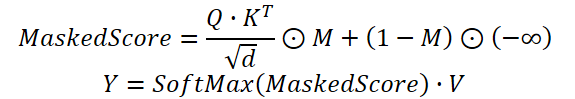
In practice, we use a modified Self-Attention mechanism, where dependency coefficients obtained from the temporal clustering module are multiplied by the mask generated by the channel clustering module. Only after that are the weights normalized using the Softmax function.
The proposed algorithm is implemented within the CNeuronDUET object, which combines the functionality of the three modules described above. The structure of the new class is shown below.
class CNeuronDUET :  public CNeuronTransposeOCL
  {
protected:
   uint                       iWindowKey;
   uint                       iHeads;
   //---
   CNeuronTransposeOCL        cTranspose;
   CNeuronMoE                 cExperts;
   CNeuronConvOCL             cQKV;
   CNeuronBaseOCL             cQ;
   CNeuronBaseOCL             cKV;
   CNeuronChanelMask          cMask;
   CBufferFloat               cbScores;
   CNeuronBaseOCL             cMHAttentionOut;
   CNeuronConvOCL             cPooling;
   CNeuronBaseOCL             cResidual;
   CNeuronMHFeedForward       cFeedForward;
   //---
   virtual bool      AttentionOut(void);
   virtual bool      AttentionInsideGradients(void);
   //---
   virtual bool      feedForward(CNeuronBaseOCL *NeuronOCL);
   virtual bool      updateInputWeights(CNeuronBaseOCL *NeuronOCL);
   virtual bool      calcInputGradients(CNeuronBaseOCL *prevLayer);

public:
                     CNeuronDUET(void) {};
                    ~CNeuronDUET(void) {};
   //---
   virtual bool      Init(uint numOutputs, uint myIndex, COpenCLMy *open_cl,
                          uint window, uint window_key, uint units_count, uint heads,
                          uint units_out, uint experts, uint top_k,
                          ENUM_OPTIMIZATION optimization_type, uint batch);
   //---
   virtual int       Type(void) override   const   {  return defNeuronDUET; }
   //---
   virtual bool      Save(int const file_handle) override;
   virtual bool      Load(int const file_handle) override;
   //---
   virtual bool      WeightsUpdate(CNeuronBaseOCL *source, float tau) override;
   virtual void      SetOpenCL(COpenCLMy *obj) override;
   //---
   virtual void      TrainMode(bool flag)
     {  bTrain = flag; cExperts.TrainMode(bTrain); }
  };
It is important to note that, in this case, the parent class is a data transposition layer. This is due to the structure of the source data.
The model takes as input a multivariate time series represented as a matrix, where each row corresponds to a separate time step of the analyzed system. However, all the modules described above operate on univariate time series. This also applies to the data fusion module. To ensure correct data processing, the input data is transposed into a format suitable for analysis. After all operations are completed, the results are transformed back into the original representation. This final step is handled by the parent class, which ensures consistency of the data structure and simplifies module integration.
In the class structure presented above, one can observe a fairly large number of internal objects that play an important role in constructing the algorithm. Their functionality will be examined in more detail during the implementation of the class virtual methods. For now, it is important to note that all objects are declared directly in the class, which allows the constructor and destructor to remain empty. Initialization of all objects, including inherited ones, is performed in the Init method.
bool CNeuronDUET::Init(uint numOutputs, uint myIndex, COpenCLMy *open_cl,
                       uint window, uint window_key, uint units_count,
                       uint heads, uint units_out, uint experts, uint top_k,
                       ENUM_OPTIMIZATION optimization_type, uint batch)
  {
   if(!CNeuronTransposeOCL::Init(numOutputs, myIndex, open_cl, window, units_out, optimization_type, batch))
      return false;
The initialization method receives a set of constants that define the architecture of the object. The structure of these parameters is already familiar. Some were used in the construction of the temporal and channel clustering modules, while others are related to attention blocks. Particular attention should be paid to the units_out parameter, which defines the desired output sequence length.
Within the method body, we first call the corresponding method of the parent class, where validation of some parameters and initialization of inherited interfaces are already implemented.
Next, the required parameters are stored in internal variables.
iWindowKey = MathMax(window_key, 1);
iHeads = MathMax(heads, 1);
We then proceed to initialize internal objects. As mentioned earlier, the input data must be transposed prior to analysis. This functionality is handled by a dedicated object.
int index = 0;
if(!cTranspose.Init(0, index, OpenCL, units_count, window, optimization, iBatch))
   return false;
After that, the temporal and channel clustering modules are initialized.
index++;
if(!cExperts.Init(0, index, OpenCL, units_count, units_out, window, experts, top_k, optimization, iBatch))
   return false;
index++;
if(!cMask.Init(0, index, OpenCL, units_count, window, optimization, iBatch))
   return false;
Next, we have the objects of the data fusion module. It essentially represents a modified attention module. First, we initialize the object responsible for generating the Query, Key, and Value entities. In this case, a single convolutional layer is used for parallel generation of all three entities.
index++;
if(!cQKV.Init(0, index, OpenCL, units_out, units_out, iHeads * iWindowKey * 3, window, 1, optimization, iBatch))
   return false;
We also add two objects for splitting these entities into separate tensors.
index++;
if(!cQ.Init(0, index, OpenCL, cQKV.Neurons() / 3, optimization, iBatch))
   return false;
index++;
if(!cKV.Init(0, index, OpenCL, cQ.Neurons() * 2, optimization, iBatch))
   return false;
Attention coefficients are stored in a data buffer.
if(!cbScores.BufferInit(cMask.Neurons()*iHeads, 0) ||
   !cbScores.BufferCreate(OpenCL))
   return false;
Note that in all cases, object dimensions are specified with consideration of the transposed input matrix.
Next, we initialize the multi-head attention output object.
index++;
if(!cMHAttentionOut.Init(0, index, OpenCL, cQ.Neurons(), optimization, iBatch))
   return false;
Then, we initialize a convolutional layer for dimensionality reduction and merging outputs from different attention heads.
index++;
if(!cPooling.Init(0, index, OpenCL, iWindowKey * iHeads, iWindowKey * iHeads, units_out, window,
                                                                        1, optimization, iBatch))
   return false;
cPooling.SetActivationFunction(None);
We then add an object to store the residual connection results.
index++;
if(!cResidual.Init(0, index, OpenCL, cPooling.Neurons(), optimization, iBatch))
   return false;
cResidual.SetActivationFunction(None);
Following the original architecture, a standard FeedForward block is expected. However, we replace it with a multi-head variant borrowed from the StockFormer framework.
   index++;
   if(!cFeedForward.Init(0, index, OpenCL, units_out, 4 * units_out, window, 1, heads, optimization, iBatch))
      return false;
//---
   return true;
  }
The method concludes by returning the logical result of the operation to the caller.
The next stage is the implementation of the forward pass in the CNeuronDUET::feedForward method.
bool CNeuronDUET::feedForward(CNeuronBaseOCL *NeuronOCL)
  {
   if(!cTranspose.FeedForward(NeuronOCL))
      return false;
The method receives a pointer to the input data object, which is immediately passed to the corresponding method of the internal data transposition object. All further operations are performed on the transposed data.
First, the data is passed to the temporal clustering module to obtain forecasts for univariate sequences.
if(!cExperts.FeedForward(cTranspose.AsObject()))
   return false;
Then, the transposed input is passed to the channel clustering module.
if(!cMask.FeedForward(cTranspose.AsObject()))
   return false;
Next, we organize the forward pass of the data fusion module. Query, Key, and Value entities are generated from the outputs of the temporal clustering module.
if(!cQKV.FeedForward(cExperts.AsObject()))
   return false;
The output is then split into two tensors.
if(!DeConcat(cQ.getOutput(), cKV.getOutput(), cQKV.getOutput(), iWindowKey, 2 * iWindowKey, cQKV.GetUnits()))
   return false;
Then, the masked multi-head Self-Attention wrapper method is invoked.
if(!AttentionOut())
   return false;
The outputs of the multi-head attention are projected to match the dimensionality of the temporal clustering module outputs.
if(!cPooling.FeedForward(cMHAttentionOut.AsObject()))
   return false;
Residual connections are then added to the obtained values.
if(!SumAndNormilize(cExperts.getOutput(), cPooling.getOutput(), cResidual.getOutput(), iWindow, true, 0, 0, 0, 1))
   return false;
The multi-head FeedForward block is implemented as a separate module with built-in residual connections. Therefore, it is sufficient to call its corresponding method, passing the results of previous operations as input.
if(!cFeedForward.FeedForward(cResidual.AsObject()))
   return false;
Finally, the results are transformed back into the original data representation. Here we use the functionality of the parent class.
 return CNeuronTransposeOCL::feedForward(cFeedForward.AsObject());
}
We return the logical result of the performed operations to the calling program and complete the execution of the method.
After completing the implementation of the feed-forward processes, we move on to the backpropagation algorithms. As you know, this involves two methods:
- Distribution of the error gradient across internal objects and input data according to their contribution to the final result — calcInputGradients
- Optimization of model parameters to minimize overall error — updateInputWeights
All trainable parameters of the DUET block in this implementation are contained within internal objects, so we just call the corresponding methods of these objects. The more critical issue is the correct distribution of the error gradient across the internal objects and the input data.
The calcInputGradients method receives a pointer to the input data object. This is the same object used during the feed-forward pass. This time, however, it must be populated with the corresponding gradient values.
bool CNeuronDUET::calcInputGradients(CNeuronBaseOCL *prevLayer)
  {
   if(!prevLayer)
      return false;
Clearly, data can only be passed to a valid object, so we immediately check the pointer validity. Otherwise, further operations would be meaningless.
As you know, gradient distribution strictly follows the information flow of the feed-forward pass, but in reverse order. Since the feed-forward pass concluded with a call to the parent class method, the backpropagation pass begins with a call to the parent class method. This time, we call the error gradient distribution method.
if(!CNeuronTransposeOCL::calcInputGradients(cFeedForward.AsObject()))
   return false;
Next, the gradient is propagated through the multi-head FeedForward module.
if(!cPooling.calcHiddenGradients(cFeedForward.AsObject()))
   return false;
Then, the resulting gradients are distributed across attention heads.
if(!cMHAttentionOut.calcHiddenGradients(cPooling.AsObject()))
   return false;
The next step is to call the wrapper method for distributing error across Query, Key, and Value within the masked Self-Attention mechanism.
if(!AttentionInsideGradients())
   return false;
The results are combined into a single tensor.
if(!Concat(cQ.getGradient(), cKV.getGradient(), cQKV.getGradient(), iWindowKey, 2 * iWindowKey, iCount))
   return false;
If necessary, the values are adjusted using the derivative of the activation function.
if(cQKV.Activation() != None)
   if(!DeActivation(cQKV.getOutput(), cQKV.getGradient(), cQKV.getGradient(), cQKV.Activation()))
      return false;
The gradient is then passed to the temporal clustering module.
if(!cExperts.calcHiddenGradients(cQKV.AsObject()) ||
   !DeActivation(cExperts.getOutput(), cExperts.getPrevOutput(), cPooling.getGradient(), cExperts.Activation()) ||
   !SumAndNormilize(cExperts.getGradient(), cExperts.getPrevOutput(), cExperts.getGradient(), iWindow, false,
                                                                                                   0, 0, 0, 1))
   return false;
It is important to note that the outputs of the temporal clustering module were also used for residual connections. Therefore, the gradient must also be propagated along this path. To achieve this, the gradient at the output of the attention block is first adjusted using the derivative of the temporal clustering module's activation function, and then gradients from both paths are summed.
Next, the gradient is propagated through the temporal clustering module.
   if(!cTranspose.calcHiddenGradients(cExperts.AsObject()))
      return false;
Finally, it is passed back to the input data level.
   return prevLayer.calcHiddenGradients(cTranspose.AsObject());
  }
We return the logical result of the performed operations to the calling program and complete the execution of the method.
Note that during gradient propagation, there is no information flow through the channel clustering module. As mentioned earlier, this module does not include a backpropagation pass, and at this stage, we simply exclude unnecessary operations.
This concludes our discussion of the algorithms implementing our interpretation of the approaches proposed by the authors of the DUET framework. The full source code of all described objects and their methods is available in the article attachments.
Model Architecture
The next stage involves integrating the developed components into the architecture of trainable models. To this end, we proceed to describe the architectural design of the models.
As in previous work, we adopt a multi-task learning approach and train two models simultaneously: the Actor model and a model for predicting the probability of the direction of future movement. The architecture of the latter is fully borrowed from previous work, so in this article we focus on the Actor architecture. The architectures of both models are presented in the CreateDescriptions method.
bool CreateDescriptions(CArrayObj *&actor, CArrayObj *&probability)
  {
//---
   CLayerDescription *descr;
//---
   if(!actor)
     {
      actor = new CArrayObj();
      if(!actor)
         return false;
     }
   if(!probability)
     {
      probability = new CArrayObj();
      if(!probability)
         return false;
     }
In the method parameters, we receive pointers to two dynamic objects intended for storing the descriptions of the model architectures. Within the method body, we immediately validate the received pointers and, if necessary, create new instances of the objects.
The Actor model architecture begins with a fully connected layer, which serves as the input data interface. It must be sufficiently large to accommodate the entire volume of analyzed information.
//--- Actor
   actor.Clear();
//--- Input layer
   if(!(descr = new CLayerDescription()))
      return false;
   descr.type = defNeuronBaseOCL;
   int prev_count = descr.count = (HistoryBars * BarDescr);
   descr.activation = None;
   descr.optimization = ADAM;
   if(!actor.Add(descr))
     {
      delete descr;
      return false;
     }
As proposed by the authors of the DUET framework, this is followed by a batch normalization layer, designed to standardize the input data and minimize the impact of outliers.
//--- layer 1
   if(!(descr = new CLayerDescription()))
      return false;
   descr.type = defNeuronBatchNormOCL;
   descr.count = prev_count;
   descr.batch = 1e4;
   descr.activation = None;
   descr.optimization = ADAM;
   if(!actor.Add(descr))
     {
      delete descr;
      return false;
     }
Next, we use two consecutive DUET blocks constructed earlier. However, the approach to data segmentation has been modified. Instead of traditional segmentation, this experiment employs a representation of data in a multidimensional phase space. This method, inspired by the Attraos framework, enables more accurate modeling of complex dependencies in time series, improving interpretability. In the first layer, a step of 5 minutes is used.
Within the temporal clustering module, 16 parallel encoders are initialized. For each cluster, the 4 most suitable ones are selected.
//--- layer 2
   if(!(descr = new CLayerDescription()))
      return false;
   descr.type = defNeuronDUET;
   descr.window = BarDescr * 5;  // 5 min
     {
      int temp[] = {HistoryBars / 5, HistoryBars / 5, 16, 4}; // {Units in (24), Units out (24), Experts, Top K}
      if(ArrayCopy(descr.units, temp) < (int)temp.Size())
         return false;
     }
   descr.window_out = 256;
   descr.step = 4;
   descr.batch = 1e4;
   descr.activation = None;
   descr.optimization = ADAM;
   if(!actor.Add(descr))
     {
      delete descr;
      return false;
     }
In the second DUET block, the phase representation step is increased to 15, while all other parameters remain unchanged.
//--- layer 3
   if(!(descr = new CLayerDescription()))
      return false;
   descr.type = defNeuronDUET;
   descr.window = BarDescr * 15;  // 15 min
     {
      int temp[] = {HistoryBars / 15, HistoryBars / 15, 16, 4}; // {Units in (8), Units out (8), Experts, Top K}
      if(ArrayCopy(descr.units, temp) < (int)temp.Size())
         return false;
     }
   descr.window_out = 256;
   descr.step = 4;
   descr.batch = 1e4;
   descr.activation = None;
   descr.optimization = ADAM;
   if(!actor.Add(descr))
     {
      delete descr;
      return false;
     }
Note that during data processing, the tensor size remains unchanged. However, the subsequent convolutional layer reduces the sequence length by a factor of three.
//--- layer 4
   if(!(descr = new CLayerDescription()))
      return false;
   descr.type = defNeuronConvOCL;
   prev_count = descr.count = HistoryBars / 3;
   descr.window = BarDescr * 3;
   descr.step = descr.window;
   int prev_window = descr.window_out = BarDescr;
   descr.activation = SoftPlus;
   descr.optimization = ADAM;
   if(!actor.Add(descr))
     {
      delete descr;
      return false;
     }
Next comes the decision-making block of 3 fully connected layers.
//--- layer 5
   if(!(descr = new CLayerDescription()))
      return false;
   descr.type = defNeuronBaseOCL;
   descr.count = LatentCount;
   descr.batch = 1e4;
   descr.activation = TANH;
   descr.optimization = ADAM;
   if(!actor.Add(descr))
     {
      delete descr;
      return false;
     }
//--- layer 6
   if(!(descr = new CLayerDescription()))
      return false;
   descr.type = defNeuronBaseOCL;
   descr.count = LatentCount;
   descr.activation = TANH;
   descr.batch = 1e4;
   descr.optimization = ADAM;
   if(!actor.Add(descr))
     {
      delete descr;
      return false;
     }
//--- layer 7
   if(!(descr = new CLayerDescription()))
      return false;
   descr.type = defNeuronBaseOCL;
   prev_count = descr.count = NActions;
   descr.activation = SoftPlus;
   descr.batch = 1e4;
   descr.optimization = ADAM;
   if(!actor.Add(descr))
     {
      delete descr;
      return false;
     }
Then comes a batch normalization layer.
//--- layer 8
   if(!(descr = new CLayerDescription()))
      return false;
   descr.type = defNeuronBatchNormOCL;
   descr.count = prev_count;
   descr.batch = 1e4;
   descr.activation = None;
   descr.optimization = ADAM;
   if(!actor.Add(descr))
     {
      delete descr;
      return false;
     }
At the output of the Actor, we add a risk management block.
//--- layer 9
   if(!(descr = new CLayerDescription()))
      return false;
   descr.type = defNeuronMacroHFTvsRiskManager;
//--- Windows
     {
      int temp[] = {3, 15, NActions, AccountDescr}; //Window, Stack Size, N Actions, Account Description
      if(ArrayCopy(descr.windows, temp) < int(temp.Size()))
         return false;
     }
   descr.count = 10;
   descr.window_out = 64;
   descr.step = 4;                              // Heads
   descr.batch = 1e4;
   descr.activation = None;
   descr.optimization = ADAM;
   if(!actor.Add(descr))
     {
      delete descr;
      return false;
     }
//--- layer 10
   if(!(descr = new CLayerDescription()))
      return false;
   descr.type = defNeuronConvOCL;
   descr.count = NActions / 3;
   descr.window = 3;
   descr.step = 3;
   descr.window_out = 3;
   descr.activation = SIGMOID;
   descr.optimization = ADAM;
   if(!actor.Add(descr))
     {
      delete descr;
      return false;
     }
The complete architecture of both models can be found in the attachments. The attachments also include environment interaction and model training programs, reused from previous work without modification.
Testing
A significant amount of work has been carried out to implement our interpretation of the approaches proposed in the DUET framework using MQL5 and to integrate them into trainable models. We can now move on to the key stage: testing the implemented solutions on real historical data.
For model training, we use a dataset of historical data for the EURUSD currency pair on the M1 timeframe for the entire year 2024. During data collection, indicator parameters are kept at their default values.
Model training is conducted in two stages. First, the batch size is set to 1, so that a random state from the training dataset is selected at each iteration. This helps the model adapt to varying conditions. However, this is not sufficient for proper functioning of the risk management block. Therefore, in the second stage, the batch size is increased to 60, allowing sequences of 60 environment states and corresponding Actor actions to be taken into account. This makes the training process more stable and efficient.
The trained model is tested on historical data from January–February 2025. All settings are preserved, ensuring an objective evaluation of forecast quality. The testing results are presented below.


During the testing period, the model executed 53 trades, more than 56% of which were closed with a profit. Notably, the average profit per winning trade is nearly twice that of losing positions. This resulted in a profit factor of 2.44.
Conclusion
In this work, we explored the DUET framework, whose authors combine frequency-domain analysis, metric learning, and probabilistic filtering for multivariate time series analysis. These components improve forecast quality and enhance model robustness to noise.
In the practical part, we implemented our interpretation of the proposed approaches using MQL5 and integrated them into a model. We trained the model on real historical data and tested it on out-of-sample data. The obtained results demonstrate the model's potential. However, before deploying it in real trading conditions, it is necessary to train the model on a more representative dataset followed by comprehensive testing.
References
Programs Used in the Article
| # | Name | Type | Description |
|---|---|---|---|
| 1 | Research.mq5 | Expert Advisor | Expert Advisor for collecting samples |
| 2 | ResearchRealORL.mq5 | Expert Advisor | Expert Advisor for collecting samples using the Real-ORL method |
| 3 | Study.mq5 | Expert Advisor | Model training Expert Advisor |
| 4 | Test.mq5 | Expert Advisor | Model Testing Expert Advisor |
| 5 | Trajectory.mqh | Class library | System state and model architecture description structure |
| 6 | NeuroNet.mqh | Class library | A library of classes for creating a neural network |
| 7 | NeuroNet.cl | Code library | OpenCL program code |
Translated from Russian by MetaQuotes Ltd.
Original article: https://www.mql5.com/ru/articles/17487
Warning: All rights to these materials are reserved by MetaQuotes Ltd. Copying or reprinting of these materials in whole or in part is prohibited.
This article was written by a user of the site and reflects their personal views. MetaQuotes Ltd is not responsible for the accuracy of the information presented, nor for any consequences resulting from the use of the solutions, strategies or recommendations described.

- Free trading apps
- Over 8,000 signals for copying
- Economic news for exploring financial markets
You agree to website policy and terms of use