Neural Networks in Trading: Multi-Task Learning Based on the ResNeXt Model (Final Part)

Introduction

In the previous article, we became familiar with the theoretical aspects of a multi-task learning framework based on the ResNeXt architecture, proposed for building financial market analysis systems. Multi-Task Learning (MTL) uses a single encoder to process the input data and multiple specialized "heads" (outputs), each designed to solve a specific task. This approach offers a number of advantages.

First, the use of a shared encoder facilitates the extraction of the most robust and universal patterns in the data that prove useful across diverse tasks. Unlike traditional approaches, where each model is trained on a separate subset of data, a multi-task architecture forms representations that capture more fundamental regularities. This makes the model more general-purpose and more resilient to noise in the raw data.

Second, joint training of multiple tasks reduces the likelihood of model overfitting. If one of the subtasks encounters low-quality or weakly informative data, the other tasks compensate for this effect through the shared encoder structure. This improves the stability and reliability of the model, especially under the highly volatile conditions of financial markets.

Third, this approach is more efficient in terms of computational resources. Instead of training several independent models that perform related functions, multi-task learning enables the use of a single encoder, reducing computational redundancy and accelerating the training process. This is particularly important in algorithmic trading, where model latency is critical for making timely trading decisions.

In the context of financial markets, MTL provides additional benefits by enabling the simultaneous analysis of multiple market factors. For example, a model can concurrently forecast volatility, identify market trends, assess risk, and incorporate the news background. The interdependence of these aspects makes multi-task learning a powerful tool for modeling complex market systems and for more accurate price dynamics forecasting.

One of the key advantages of multi-task learning is its ability to dynamically shift priorities among different subtasks. This means that the model can adapt to changes in the market environment, focusing more on the aspects that have the greatest impact on current price movements.

The ResNeXt architecture, chosen by the framework authors as the basis for the encoder, is characterized by its modularity and high efficiency. It uses grouped convolutions, which significantly improve model performance without a substantial increase in computational complexity. This is especially important for processing large streams of market data in real time. The flexibility of the architecture also allows model parameters to be tailored to specific tasks: varying network depth, convolutional block configurations, and data normalization methods, making it possible to adapt the system to different operating conditions.

The combination of multi-task learning and the ResNeXt architecture yields a powerful analytical tool capable of efficiently integrating and processing diverse information sources. This approach not only improves forecast accuracy but also allows the system to rapidly adapt to market changes, uncovering hidden dependencies and patterns. Automatic extraction of significant features makes the model more robust to anomalies and helps minimize the impact of random market noise.

In the practical part of the previous article, we examined in detail the implementation of the key components of the ResNeXt architecture using MQL5. During this work, a grouped convolution module with a residual connection was created, implemented as the CNeuronResNeXtBlock object. This approach ensures high system flexibility, scalability, and efficiency in processing financial data.

In the present work, we move away from creating the encoder as a monolithic object. Instead, users will be able to construct the encoder architecture themselves, using the already implemented building blocks. This will not only provide greater flexibility but will also expand the system's ability to adapt to various types of financial data and trading strategies. Today, the primary focus will be on the development and training of models within the multi-task learning framework.

Model Architecture

Before proceeding with the technical implementation, it is necessary to define the key tasks solved by the models. One of them will perform the role of an Agent, responsible for generating the parameters of trading operations. It will produce trade parameters, similar to the architectures discussed earlier. This approach helps avoid excessive duplication of computations, improves the consistency of forecasts, and establishes a unified decision-making strategy.

However, such a structure does not fully employ the potential of multi-task learning. To achieve the desired effect, an additional model will be added to the system, trained to forecast future market trends. This predictive block will improve forecast accuracy and enhance the model's resilience to sudden market changes. Under conditions of high market volatility, this mechanism enables the model to quickly adapt to new information and make more precise trading decisions.

Integrating multiple tasks into a single model will create a comprehensive analytical system capable of accounting for numerous market factors and interacting with them in real time. This approach is expected to provide a higher degree of knowledge generalization, improve forecast accuracy, and minimize risks associated with erroneous trading decisions.

The architecture of the trained models is defined in the CreateDescriptions method. The method parameters include two pointers to dynamic array objects, into which the model architectures will be written.

bool CreateDescriptions(CArrayObj *&actor, CArrayObj *&probability)
  {
//---
   CLayerDescription *descr;
//---
   if(!actor)
     {
      actor = new CArrayObj();
      if(!actor)
         return false;
     }
   if(!probability)
     {
      probability = new CArrayObj();
      if(!probability)
         return false;
     }

A key implementation feature is the creation of two specialized models: the Actor and a predictive model responsible for the probabilistic assessment of the upcoming price movement direction. The environment state Encoder is integrated directly into the Actor architecture, allowing it to form rich representations of market data and capture complex dependencies. In turn, the second model receives its input from the Actor's latent space, using its learned representations to generate more accurate predictions. This approach not only improves forecasting efficiency but also reduces computational load, ensuring coordinated operation of both models within a unified system.

In the method body, we first verify the validity of the received pointers and, if necessary, create new instances of the dynamic array objects.

Next, we proceed to build the architecture of the Actor, starting with the environment encoder. The first component is a base neural layer used to record the raw input data. The size of this layer is determined by the volume of the analyzed data.

//--- Actor
   actor.Clear();
//--- Input layer
   if(!(descr = new CLayerDescription()))
      return false;
   descr.type = defNeuronBaseOCL;
   int prev_count = descr.count = (HistoryBars * BarDescr);
   descr.activation = None;
   descr.optimization = ADAM;
   if(!actor.Add(descr))
     {
      delete descr;
      return false;
     }

No activation functions are applied, since, in essence, the output buffer of this layer directly stores the raw data obtained from the environment. In our case, these data are received directly from the terminal, which allows their original structure to be preserved. However, this approach has a significant drawback: the lack of preprocessing can negatively affect the model's trainability, as the raw data contain heterogeneous values that differ in scale and distribution.

To mitigate this issue, a batch normalization mechanism is applied immediately after the first layer. It performs preliminary data standardization, bringing the inputs to a common scale and improving their comparability. This significantly enhances training stability, accelerates model convergence, and reduces the risk of gradient explosion or vanishing. As a result, even when working with highly volatile market data, the model gains the ability to form more accurate and consistent representations, which is critically important for subsequent multi-task analysis.

//--- layer 1
   if(!(descr = new CLayerDescription()))
      return false;
   descr.type = defNeuronBatchNormOCL;
   descr.count = prev_count;
   descr.batch = 1e4;
   descr.activation = None;
   descr.optimization = ADAM;
   if(!actor.Add(descr))
     {
      delete descr;
      return false;
     }

Next, we use a convolutional layer that transforms the feature space, bringing it to a standardized dimensionality. This makes it possible to create a unified data representation, ensuring consistency at subsequent processing stages. The Leaky ReLU (LReLU) activation function is used, which helps reduce the influence of minor fluctuations and random noise while preserving the important characteristics of the original data.

//--- layer 2
   if(!(descr = new CLayerDescription()))
      return false;
   descr.type = defNeuronConvOCL;
   descr.count = HistoryBars;
   descr.window = BarDescr;
   descr.step = BarDescr;
   descr.window_out = 128;
   descr.activation = LReLU;
   descr.optimization = ADAM;
   if(!actor.Add(descr))
     {
      delete descr;
      return false;
     }

After completing the preliminary data preprocessing, we proceed to designing the architecture of the environment state Encoder, which plays a key role in analyzing and interpreting the raw input data. The primary objective of the Encoder is to identify stable patterns and hidden structures within the analyzed dataset, enabling the formation of an informative representation for subsequent processing by decision-making models.

Our Encoder is built from three sequential ResNeXt architecture blocks, each of which uses grouped convolutions for efficient feature extraction. In each block, a convolutional filter is applied with a window size of 3 elements of the analyzed multidimensional time series and a convolution stride of 2 elements. This ensures that the dimensionality of the original sequence is halved in each block.

//--- layer 3
   if(!(descr = new CLayerDescription()))
      return false;
   descr.type = defNeuronResNeXtBlock;
//--- Chanels
     {
      int temp[] = {128, 256}; //In, Out
      if(ArrayCopy(descr.windows, temp) < int(temp.Size()))
         return false;
     }
//--- Units and Groups
     {
      int temp[] = {HistoryBars, 4, 32}; //Units, Group Size, Groups
      if(ArrayCopy(descr.units, temp) < int(temp.Size()))
         return false;
     }
   descr.window = 3;
   descr.step = 2;
   descr.window_out = 1;
   descr.batch = 1e4;
   descr.activation = None;
   descr.optimization = ADAM;
   if(!actor.Add(descr))
     {
      delete descr;
      return false;
     }
   int units_out = (descr.units[0] - descr.window + descr.step - 1) / descr.step + 1;

In accordance with the principles of the ResNeXt architecture, the reduction in the dimensionality of the analyzed multidimensional time series is compensated by a proportional increase in feature dimensionality. This approach preserves the informativeness of the data while providing a more detailed representation of the structural characteristics of the time series.

//--- layer 4
   if(!(descr = new CLayerDescription()))
      return false;
   descr.type = defNeuronResNeXtBlock;
//--- Chanels
     {
      int temp[] = {256, 512}; //In, Out
      if(ArrayCopy(descr.windows, temp) < int(temp.Size()))
         return false;
     }
//--- Units and Groups
     {
      int temp[] = {units_out, 4, 64}; //Units, Group Size, Groups
      if(ArrayCopy(descr.units, temp) < int(temp.Size()))
         return false;
     }
   descr.window = 3;
   descr.step = 2;
   descr.window_out = 1;
   descr.batch = 1e4;
   descr.activation = None;
   descr.optimization = ADAM;
   if(!actor.Add(descr))
     {
      delete descr;
      return false;
     }
   units_out = (descr.units[0] - descr.window + descr.step - 1) / descr.step + 1;

In addition, as the dimensionality of the feature space increases, we proportionally expand the number of convolution groups while keeping the size of each group fixed. This allows the architecture to scale efficiently, maintaining a balance between computational complexity and the model's ability to extract complex patterns from the data.

//--- layer 4
   if(!(descr = new CLayerDescription()))
      return false;
   descr.type = defNeuronResNeXtBlock;
//--- Chanels
     {
      int temp[] = {256, 512}; //In, Out
      if(ArrayCopy(descr.windows, temp) < int(temp.Size()))
         return false;
     }
//--- Units and Groups
     {
      int temp[] = {units_out, 4, 64}; //Units, Group Size, Groups
      if(ArrayCopy(descr.units, temp) < int(temp.Size()))
         return false;
     }
   descr.window = 3;
   descr.step = 2;
   descr.window_out = 1;
   descr.batch = 1e4;
   descr.activation = None;
   descr.optimization = ADAM;
   if(!actor.Add(descr))
     {
      delete descr;
      return false;
     }
   units_out = (descr.units[0] - descr.window + descr.step - 1) / descr.step + 1;

After three ResNeXt blocks, the feature dimensionality increases to 1024, with a proportional reduction in the length of the analyzed sequence.

//--- layer 5
   if(!(descr = new CLayerDescription()))
      return false;
   descr.type = defNeuronResNeXtBlock;
//--- Chanels
     {
      int temp[] = {512, 1024}; //In, Out
      if(ArrayCopy(descr.windows, temp) < int(temp.Size()))
         return false;
     }
//--- Units and Groups
     {
      int temp[] = {units_out, 4, 128}; //Units, Group Size, Groups
      if(ArrayCopy(descr.units, temp) < int(temp.Size()))
         return false;
     }
   descr.window = 3;
   descr.step = 2;
   descr.window_out = 1;
   descr.batch = 1e4;
   descr.activation = None;
   descr.optimization = ADAM;
   if(!actor.Add(descr))
     {
      delete descr;
      return false;
     }
   units_out = (descr.units[0] - descr.window + descr.step - 1) / descr.step + 1;

Next, the ResNeXt architecture provides for compressing the analyzed sequence along the time dimension, retaining only the most significant characteristics of the analyzed environment state. For this, we first transpose the resulting data:

//--- layer 6
   if(!(descr = new CLayerDescription()))
      return false;
   descr.type = defNeuronTransposeOCL;
   descr.count = units_out;
   descr.window = 1024;
   descr.batch = 1e4;
   descr.activation = None;
   descr.optimization = ADAM;
   if(!actor.Add(descr))
     {
      delete descr;
      return false;
     }

Then, we use a pooling layer, which reduces the dimensionality of the data while preserving the most important characteristics. This enables the model to focus on key features, eliminating unnecessary noise and providing a more compact representation of the original data.

//--- layer 7
   if(!(descr = new CLayerDescription()))
      return false;
   descr.type = defNeuronProofOCL;
   descr.count = 1024;
   descr.step = descr.window = units_out;
   descr.batch = 1e4;
   descr.activation = None;
   descr.optimization = ADAM;
   if(!actor.Add(descr))
     {
      delete descr;
      return false;
     }

Remember the ordinal number of this layer. This is the final layer of our environment state Encoder, and it is from this layer that we will take the input data for the second model.

Next comes the Decoder of our Agent, consisting of two sequential fully connected layers.

//--- layer 8
   if(!(descr = new CLayerDescription()))
      return false;
   descr.type = defNeuronBaseOCL;
   descr.count = 256;
   descr.activation = SIGMOID;
   descr.batch = 1e4;
   descr.optimization = ADAM;
   if(!actor.Add(descr))
     {
      delete descr;
      return false;
     }
//--- layer 9
   if(!(descr = new CLayerDescription()))
      return false;
   descr.type = defNeuronBaseOCL;
   descr.count = NActions;
   descr.activation = SIGMOID;
   descr.batch = 1e4;
   descr.optimization = ADAM;
   if(!actor.Add(descr))
     {
      delete descr;
      return false;
     }

Both layers use the sigmoid function as the activation function and gradually reduce the tensor dimensionality to the predefined action space of the Agent.

It should be noted here that the Agent created above analyzes only the raw environment state and is completely devoid of a risk management module. We compensate for this limitation by adding a risk management Agent layer, implemented within the MacroHFT framework.

//--- layer 10
   if(!(descr = new CLayerDescription()))
      return false;
   descr.type = defNeuronMacroHFTvsRiskManager;
//--- Windows
     {
      int temp[] = {3, 15, NActions, AccountDescr}; //Window, Stack Size, N Actions, Account Description
      if(ArrayCopy(descr.windows, temp) < int(temp.Size()))
         return false;
     }
   descr.count = 10;
   descr.window_out = 16;
   descr.step = 4;                              // Heads
   descr.batch = 1e4;
   descr.activation = None;
   descr.optimization = ADAM;
   if(!actor.Add(descr))
     {
      delete descr;
      return false;
     }

We also add a convolutional layer with a sigmoid activation function, which maps the Agent's outputs into the specified value space. We use a convolution window of size 3, which corresponds to the parameters of a single trade. This approach makes it possible to obtain consistent trade characteristics.

//--- layer 11
   if(!(descr = new CLayerDescription()))
      return false;
   descr.type = defNeuronConvOCL;
   descr.count = NActions / 3;
   descr.window = 3;
   descr.step = 3;
   descr.window_out = 3;
   descr.activation = SIGMOID;
   descr.optimization = ADAM;
   if(!actor.Add(descr))
     {
      delete descr;
      return false;
     }

At the next stage, we move on to describing the model for forecasting the probabilities of upcoming price movements. As mentioned above, our predictive model receives its input data from the Agent's latent state. To ensure dimensional consistency between the latent state and the input layer of the second model, we decided to abandon manual architectural adjustments. Instead, we extract the description of the latent state layer from the Agent's architecture description. 

//--- Probability
   probability.Clear();
//--- Input layer
   CLayerDescription *latent = actor.At(LatentLayer);
   if(!latent)
      return false;

The parameters of the extracted latent state description are then transferred to the input layer of the new model.

   if(!(descr = new CLayerDescription()))
      return false;
   descr.type = defNeuronBaseOCL;
   prev_count = descr.count = latent.count;
   descr.activation = latent.activation;
   descr.optimization = ADAM;
   if(!probability.Add(descr))
     {
      delete descr;
      return false;
     }

Using the latent state of another model as input data allows us to work with already processed and mutually comparable data. Consequently, there is no need to apply a batch normalization layer for primary input preprocessing. Moreover, the outputs of the ResNeXt blocks are already normalized.

To obtain predictive values for the forthcoming price movement direction, we use two sequential fully connected layers with a sigmoid activation function between them.

//--- layer 1
   if(!(descr = new CLayerDescription()))
      return false;
   descr.type = defNeuronBaseOCL;
   descr.count = 256;
   descr.activation = SIGMOID;
   descr.batch = 1e4;
   descr.optimization = ADAM;
   if(!probability.Add(descr))
     {
      delete descr;
      return false;
     }
//--- layer 2
   if(!(descr = new CLayerDescription()))
      return false;
   descr.type = defNeuronBaseOCL;
   prev_count = descr.count = NActions / 3;
   descr.activation = None;
   descr.batch = 1e4;
   descr.optimization = ADAM;
   if(!probability.Add(descr))
     {
      delete descr;
      return false;
     }

The outputs of the fully connected layers are then mapped into a probabilistic space using the SoftMax function.

//--- layer 3
   if(!(descr = new CLayerDescription()))
      return false;
   descr.type = defNeuronSoftMaxOCL;
   prev_count = descr.count = prev_count;
   descr.step = 1;
   descr.activation = None;
   descr.batch = 1e4;
   descr.optimization = ADAM;
   if(!probability.Add(descr))
     {
      delete descr;
      return false;
     }
//---
   return true;
  }

It is important to note that our model predicts probabilities for only two directions of price movement: upward and downward. The probability of flat (sideways) movement is deliberately not considered, since even a sideways market in practice represents a sequence of short-term price fluctuations with approximately equal amplitude and opposite directions. This approach allows the model to focus on identifying fundamental dynamic market patterns without wasting computational resources on describing complex but less significant flat states.

After completing the description of the model architectures, all that remains is to return the logical result of the performed operations to the calling program and terminate the method execution.

Model Training

Now that we have defined the model architectures, we can move on to the next stage — training. For this purpose, we will use the training dataset collected during the development of the MacroHFT framework. The dataset construction process is described in detail in the corresponding article. Let me remind you that this training dataset was built using historical data of the EURUSD currency pair for the entire year 2024 on the M1 timeframe.

However, to train the models, we need to introduce several modifications to the Expert Advisor algorithm located at ...\MQL5\Experts\ResNeXt\Study.mq5. Within the scope of this article, we will focus exclusively on the Train method, since it is where the entire training process is organized.

void Train(void)
  {
//---
   vector<float> probability = vector<float>::Full(Buffer.Size(), 1.0f / Buffer.Size());

At the beginning of the training method, we usually compute probability vectors for selecting different trajectories based on their profitability. This makes it possible to correct the imbalance between profitable and unprofitable episodes, since in most cases the number of losing sequences significantly exceeds the number of profitable ones. However, in the present work, the models are planned to be trained on nearly ideal trajectories, where the sequence of the agent's actions is formed in accordance with historical price movement data. As a result, the probability vector is filled with equal values, ensuring uniform representation of the entire training dataset. This approach allows the model to learn the key characteristics of market data without artificially biasing priorities toward certain scenarios at the expense of others. This improves generalization capability and model robustness.

Next, we declare a number of local variables required for temporary data storage during the execution of operations.

   vector<float> result, target, state;
   matrix<float> fstate = matrix<float>::Zeros(1, NForecast * BarDescr);
   bool Stop = false;
//---
   uint ticks = GetTickCount();

This concludes the preparatory work. We then proceed to create the system of training loops for the models.

It should be noted that the ResNeXt architecture itself does not use recurrent blocks. Therefore, for its training, it is reasonable to apply learning within a single loop of random state sampling from the training dataset. However, we have added a risk management agent that uses memory modules of past decisions and changes in account state resulting from their execution. Training this module requires preserving the historical sequence of the input data.

In the body of the outer loop, we sample the initial state of a mini-batch historical sequence from the training dataset.

   for(int iter = 0; (iter < Iterations && !IsStopped() && !Stop); iter += Batch)
     {
      int tr = SampleTrajectory(probability);
      int start = (int)((MathRand() * MathRand() / MathPow(32767, 2)) * 
                            (Buffer[tr].Total - 2 - NForecast - Batch));
      if(start <= 0)
        {
         iter -= Batch;
         continue;
        }

We then clear the memory of recurrent blocks.

      if(!Actor.Clear())
        {
         PrintFormat("%s -> %d", __FUNCTION__, __LINE__);
         Stop = true;
         break;
        }

Next, we fill the vector of previous target values of the Agent's actions with zero values, and then run a nested loop through the mini-batch states following their historical sequence.

      result = vector<float>::Zeros(NActions);
      for(int i = start; i < MathMin(Buffer[tr].Total, start + Batch); i++)
        {
         if(!state.Assign(Buffer[tr].States[i].state) ||
            MathAbs(state).Sum() == 0 ||
            !bState.AssignArray(state))
           {
            iter -= Batch + start - i;
            break;
           }

In the body of the nested loop, we first transfer the descriptions of the environment state from the training dataset to the corresponding buffer. After that, we move on to the formation of the tensor describing the account state. Here we generate the harmonics of the timestamp corresponding to the analyzed environment state.

         //---
         bTime.Clear();
         double time = (double)Buffer[tr].States[i].account[7];
         double x = time / (double)(D'2024.01.01' - D'2023.01.01');
         bTime.Add((float)MathSin(x != 0 ? 2.0 * M_PI * x : 0));
         x = time / (double)PeriodSeconds(PERIOD_MN1);
         bTime.Add((float)MathCos(x != 0 ? 2.0 * M_PI * x : 0));
         x = time / (double)PeriodSeconds(PERIOD_W1);
         bTime.Add((float)MathSin(x != 0 ? 2.0 * M_PI * x : 0));
         x = time / (double)PeriodSeconds(PERIOD_D1);
         bTime.Add((float)MathSin(x != 0 ? 2.0 * M_PI * x : 0));
         if(bTime.GetIndex() >= 0)
            bTime.BufferWrite();

We extract balance and equity data from the experience replay buffer.

         //--- Account
         float PrevBalance = Buffer[tr].States[MathMax(i - 1, 0)].account[0];
         float PrevEquity = Buffer[tr].States[MathMax(i - 1, 0)].account[1];

We also calculate the profitability of the last target trading operation that we could potentially have obtained on the previous historical bar.

         float profit = float(bState[0] / _Point * (result[0] - result[3]));

When preparing the account state description vector, we assume that on the previous bar all existing open positions were closed and a potential trade of the target operation, formed in the previous iteration of the nested training loop, was executed. It is easy to see that on the first iteration of this loop, the target action vector is filled with zero values (i.e., no trading operation). Consequently, the balance change coefficient is equal to "1", and the equity indicators are formed based on the potential profit of the last bar, calculated earlier.

         bAccount.Clear();
         bAccount.Add(1);
         bAccount.Add((PrevEquity + profit) / PrevEquity);
         bAccount.Add(profit / PrevEquity);
         bAccount.Add(MathMax(result[0] - result[3], 0));
         bAccount.Add(MathMax(result[3] - result[0], 0));
         bAccount.Add((bAccount[3] > 0 ? profit / PrevEquity : 0));
         bAccount.Add((bAccount[4] > 0 ? profit / PrevEquity : 0));
         bAccount.Add(0);
         bAccount.AddArray(GetPointer(bTime));
         if(bAccount.GetIndex() >= 0)
            bAccount.BufferWrite();

Accordingly, information about open positions is also formed based on the target trading operation.

After forming the input data, we perform a feed-forward pass of the trained models. First, we call the forward-pass method of the Agent, passing the input data prepared above.

         //--- Feed Forward
         if(!Actor.feedForward((CBufferFloat*)GetPointer(bState), 1, false, GetPointer(bAccount)))
           {
            PrintFormat("%s -> %d", __FUNCTION__, __LINE__);
            Stop = true;
            break;
           }

Then, we call the corresponding method of the predictive model for the probabilities of the upcoming price movement, using the Agent's latent state as the input data.

         if(!Probability.feedForward(GetPointer(Actor), LatentLayer, (CBufferFloat*)NULL))
           {
            PrintFormat("%s -> %d", __FUNCTION__, __LINE__);
            Stop = true;
            break;
           }

The next step is to generate target values for training the models. As mentioned above, we plan to train the models under "near-perfect trajectories". Therefore, the target values are formed by "looking into the future" using the data from our training dataset. To do this, we extract the actual subsequent historical environment state data from the training dataset over a given planning horizon and transfer them into a matrix, where each bar is represented by a separate row.

         //--- Look for target
         target = vector<float>::Zeros(NActions);
         bActions.AssignArray(target);
         if(!state.Assign(Buffer[tr].States[i + NForecast].state) ||
            !state.Resize(NForecast * BarDescr) ||
            MathAbs(state).Sum() == 0)
           {
            iter -= Batch + start - i;
            break;
           }
         if(!fstate.Resize(1, NForecast * BarDescr) ||
            !fstate.Row(state, 0) ||
            !fstate.Reshape(NForecast, BarDescr))
           {
            iter -= Batch + start - i;
            break;
           }

It should be noted that the extracted data are ordered in reverse historical sequence. Therefore, we organize a loop to reorder the rows of this matrix.

         for(int j = 0; j < NForecast / 2; j++)
           {
            if(!fstate.SwapRows(j, NForecast - j - 1))
              {
               PrintFormat("%s -> %d", __FUNCTION__, __LINE__);
               Stop = true;
               break;
              }
           }

Now, having data on the upcoming price movement, we proceed to forming the target trading operation vector. At this stage, the algorithm branches depending on the previous trading operation. In other words, the previous trading operation changes the Agent's target at this stage. And this is quite logical. When there is an open position, we search for an exit point; when there is none, we search for an entry point.

If, in the previous iteration, the target operation was opening a long position, we check whether the stop loss level is reached in the foreseeable future.

         target = fstate.Col(0).CumSum();
         if(result[0] > result[3])
           {
            float tp = 0;
            float sl = 0;
            float cur_sl = float(-(result[2] > 0 ? result[2] : 1) * MaxSL * Point());
            int pos = 0;
            for(int j = 0; j < NForecast; j++)
              {
               tp = MathMax(tp, target[j] + fstate[j, 1] - fstate[j, 0]);
               pos = j;
               if(cur_sl >= target[j] + fstate[j, 2] - fstate[j, 0])
                  break;
               sl = MathMin(sl, target[j] + fstate[j, 2] - fstate[j, 0]);
              }

In this case, the maximum price up to the moment when the stop loss level is reached is used as the target take profit value.

The obtained values are transferred as parameters of the target buy operation, while the parameters of the sell operation are simultaneously reset to zero.

            if(tp > 0)
              {
               sl = float(MathMin(MathAbs(sl) / (MaxSL * Point()), 1));
               tp = float(MathMin(tp / (MaxTP * Point()), 1));
               result[0] = MathMax(result[0] - result[3], 0.011f);
               result[1] = tp;
               result[2] = sl;
               for(int j = 3; j < NActions; j++)
                  result[j] = 0;
               bActions.AssignArray(result);
              }
           }

Analogous operations are performed when searching for an exit point from a short position.

         else
           {
            if(result[0] < result[3])
              {
               float tp = 0;
               float sl = 0;
               float cur_sl = float((result[5] > 0 ? result[5] : 1) * MaxSL * Point());
               int pos = 0;
               for(int j = 0; j < NForecast; j++)
                 {
                  tp = MathMin(tp, target[j] + fstate[j, 2] - fstate[j, 0]);
                  pos = j;
                  if(cur_sl <= target[j] + fstate[j, 1] - fstate[j, 0])
                     break;
                  sl = MathMax(sl, target[j] + fstate[j, 1] - fstate[j, 0]);
                 }
               if(tp < 0)
                 {
                  sl = float(MathMin(MathAbs(sl) / (MaxSL * Point()), 1));
                  tp = float(MathMin(-tp / (MaxTP * Point()), 1));
                  result[3] = MathMax(result[3] - result[0], 0.011f);
                  result[4] = tp;
                  result[5] = sl;
                  for(int j = 0; j < 3; j++)
                     result[j] = 0;
                  bActions.AssignArray(result);
                 }
              }

If there is no open position, we search for an entry point. To do this, we determine the direction of the upcoming price trend.

               ulong argmin = target.ArgMin();
               ulong argmax = target.ArgMax();
               while(argmax > 0 && argmin > 0)
                 {
                  if(argmax < argmin && target[argmax]/2 > MathAbs(target[argmin]))
                     break;
                  if(argmax > argmin && target[argmax] < MathAbs(target[argmin]/2))
                     break;
                  target.Resize(MathMin(argmax, argmin));
                  argmin = target.ArgMin();
                  argmax = target.ArgMax();
                 }

In the case of an expected upward price movement, we define the parameters of a buy trade. The parameters of the trading operation are determined similarly to the exit point search. Stop loss is set at the level of the maximum value.

               if(argmin == 0 || (argmax < argmin && argmax > 0))
                 {
                  float tp = 0;
                  float sl = 0;
                  float cur_sl = - float(MaxSL * Point());
                  ulong pos = 0;
                  for(ulong j = 0; j < argmax; j++)
                    {
                     tp = MathMax(tp, target[j] + fstate[j, 1] - fstate[j, 0]);
                     pos = j;
                     if(cur_sl >= target[j] + fstate[j, 2] - fstate[j, 0])
                        break;
                     sl = MathMin(sl, target[j] + fstate[j, 2] - fstate[j, 0]);
                    }
                  if(tp > 0)
                    {
                     sl = (float)MathMax(MathMin(MathAbs(sl) / (MaxSL * Point()), 1), 0.01);
                     tp = (float)MathMin(tp / (MaxTP * Point()), 1);
                     result[0] = float(MathMax(Buffer[tr].States[i].account[0]/100*0.01, 0.011));
                     result[1] = tp;
                     result[2] = sl;
                     for(int j = 3; j < NActions; j++)
                        result[j] = 0;
                     bActions.AssignArray(result);
                    }
                 }

Similarly, we determine the parameters of a sell trade in the case of a downward price movement.

               else
                 {
                  if(argmax == 0 || argmax > argmin)
                    {
                     float tp = 0;
                     float sl = 0;
                     float cur_sl = float(MaxSL * Point());
                     ulong pos = 0;
                     for(ulong j = 0; j < argmin; j++)
                       {
                        tp = MathMin(tp, target[j] + fstate[j, 2] - fstate[j, 0]);
                        pos = j;
                        if(cur_sl <= target[j] + fstate[j, 1] - fstate[j, 0])
                           break;
                        sl = MathMax(sl, target[j] + fstate[j, 1] - fstate[j, 0]);
                       }
                     if(tp < 0)
                       {
                        sl = (float)MathMax(MathMin(MathAbs(sl) / (MaxSL * Point()), 1), 0.01);
                        tp = (float)MathMin(-tp / (MaxTP * Point()), 1);
                        result[3] = float(MathMax(Buffer[tr].States[i].account[0]/100*0.01,0.011));
                        result[4] = tp;
                        result[5] = sl;
                        for(int j = 0; j < 3; j++)
                           result[j] = 0;
                        bActions.AssignArray(result);
                       }
                    }
                 }
              }
           }

After forming the target tensor of a trading operation, we can perform backpropagation operations of our Agent in order to minimize the deviation of the generated trading decision from the target one.

         //--- Actor Policy
         if(!Actor.backProp(GetPointer(bActions), (CBufferFloat*)GetPointer(bAccount),
                                                               GetPointer(bGradient)))
           {
            PrintFormat("%s -> %d", __FUNCTION__, __LINE__);
            Stop = true;
            break;
           }

Next, we need to formulate the target values for the predictive model. I think it is obvious that a buy trade corresponds to an uptrend, and a sell trade corresponds to a downtrend. Since the trades are formed based on the analysis of historical data, we have 100% confidence in the upcoming trend. Therefore, the target value for the corresponding trend is 1 and 0 for the opposite one.

         target = vector<float>::Zeros(NActions / 3);
         for(int a = 0; a < NActions; a += 3)
            target[a / 3] = float(result[a] > 0);

Now we can run backpropagation operations on the predictive model as well. In doing so, we adjust the parameters of the environment state encoder, which is consistent with multi-task learning approaches.

         if(!Result.AssignArray(target) ||
            !Probability.backProp(Result, GetPointer(Actor), LatentLayer) ||
            !Actor.backPropGradient((CBufferFloat*)NULL, (CBufferFloat*)NULL, LatentLayer))
           {
            PrintFormat("%s -> %d", __FUNCTION__, __LINE__);
            Stop = true;
            break;
           }

Now we just need to inform the user about the progress of the learning process and move on to the next iteration of the loop system.

         if(GetTickCount() - ticks > 500)
           {
            double percent = double(iter + i - start) * 100.0 / (Iterations);
            string str = StringFormat("%-14s %6.2f%% -> Error %15.8f\n", "Actor",
                                         percent, Actor.getRecentAverageError());
            str += StringFormat("%-13s %6.2f%% -> Error %15.8f\n", "Probability", 
                                   percent, Probability.getRecentAverageError());
            Comment(str);
            ticks = GetTickCount();
           }
        }
     }

After successfully completing a specified number of training iterations, we clear the chart comments, through which we informed the user about the model training progress.

   Comment("");
//---
   PrintFormat("%s -> %d -> %-15s %10.7f", __FUNCTION__, __LINE__,
                          "Actor", Actor.getRecentAverageError());
   PrintFormat("%s -> %d -> %-15s %10.7f", __FUNCTION__, __LINE__, 
              "Probability", Probability.getRecentAverageError());
   ExpertRemove();
//---
  }

We output the training results to the log and initialize the training program termination process. You can find the full code of the model training program in the attachment.

The next step is to proceed directly to the model training process. For this purpose, we switch to the MetaTrader 5 terminal and launch the created Expert Advisor in real-time mode. The EA does not execute any trading operations, so its operation poses no risk to the account balance.

It should be noted that we perform simultaneous training of both models. However, there is one nuance in the operation of the Agent. As mentioned above, a risk management block was added to the architecture of this model, using memory modules of the account state and past decisions. At the same time, information from the Agent's latent representation is stored in the memory module of previous actions.

However, if we refer to the training code presented above, we can see that the account state description vector is formed based on target values. This creates an imbalance: the risk management block evaluates balance changes in the context of a completely different behavior policy. To minimize this effect, I decided to conduct training in two stages.

At the first training stage, we set the mini-batch size equal to a single state.

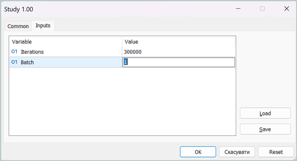
Such a parameter configuration effectively disables the memory modules during the first training stage. This is, of course, not the target operating mode of our model, but in this mode we can bring the Agent's behavior policy as close as possible to the target one, minimizing the gap between predicted and target trading operations.

At the second training stage, we increase the mini-batch size, setting it at least slightly larger than the capacity of the memory modules. This allows us to fine-tune the model, including the operation of the risk management component that controls the impact of the chosen policy on the account state.

Model Testing

After training the models, we move on to testing the resulting Agent behavior policy. Here, it is necessary to briefly mention the changes introduced into the testing program algorithm. These adjustments are local in nature. So we will not review the entire code, which you can examine independently in the attachment. We will only note that we added our probability forecasting model of upcoming price movement to the program logic. A trading operation is executed only if the direction of the Agent's trading operation coincides with the most probable trend.

We test the trained policy in the MetaTrader 5 Strategy Tester using historical data from January 2025, while fully preserving all other parameters used for assembling the training dataset. The test period was not included in the training dataset. This makes the testing conditions as close as possible to real-world operation on unseen data.

The test results are presented below.

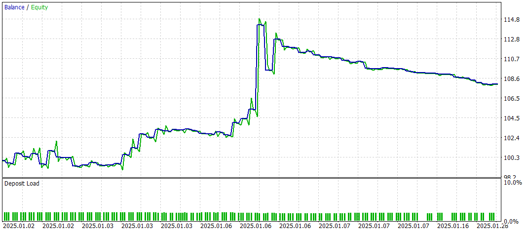
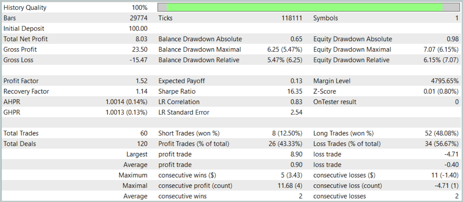
During the testing period, the model executed 60 trading operations, which averages to about 3 trades per trading day. More than 43% of the opened positions were closed with a profit. Due to the fact that the average and maximum profitable trades were almost twice as large as the corresponding metrics of losing trades, the testing concluded with a positive financial result. The profit factor was recorded at 1.52, while the recovery factor reached 1.14.

Conclusion

The multi-task learning framework based on the ResNeXt architecture discussed in this article opens up new opportunities for financial market analysis. Thanks to the use of a shared encoder and specialized "heads", the model is able to effectively identify stable patterns in data, adapt to changing market conditions, and deliver more accurate forecasts. The application of multi-task learning helps minimize the risk of overfitting, as the model is trained on several tasks simultaneously, contributing to the formation of more generalized market representations.

In addition, the high modularity of the ResNeXt architecture enables the tuning of model parameters depending on specific operating conditions, making it a versatile tool for algorithmic trading.

The presented implementation of our interpretation of the proposed approaches using MQL5 has demonstrated effectiveness in time series analysis and market trend forecasting. The inclusion of an additional market trend forecasting block significantly enhanced the analytical capabilities of the model, making it more resilient to unexpected price changes.

Overall, the proposed system demonstrates significant potential for application in automated trading and algorithmic analysis of financial data. However, before deploying the model in real market conditions, it must be trained on a more representative training dataset followed by comprehensive testing.

References

• Aggregated Residual Transformations for Deep Neural Networks
• Collaborative Optimization in Financial Data Mining Through Deep Learning and ResNeXt
• Other articles from this series

Programs used in the article

#	Name	Type	Description
1	Research.mq5	Expert Advisor	Expert Advisor for collecting samples
2	ResearchRealORL.mq5	Expert Advisor	Expert Advisor for collecting samples using the Real-ORL method
3	Study.mq5	Expert Advisor	Model training Expert Advisor
4	Test.mq5	Expert Advisor	Model testing Expert Advisor
5	Trajectory.mqh	Class library	System state and model architecture description structure
6	NeuroNet.mqh	Class library	A library of classes for creating a neural network
7	NeuroNet.cl	Code Base	OpenCL program code