Data Science and ML (Part 40): Using Fibonacci Retracements in Machine Learning data

MetaTrader 5 — Expert Advisors | 15 May 2025, 15:12

596

Omega J Msigwa

Contents

The Origin of Fibonacci Numbers

Fibonacci numbers can be traced back to the ancient mathematician Leonardo of Pisa, also known as Fibonacci.

In his book named "Liber Abaci", published in 1202, Fibonacci introduced the sequence of numbers now known as the Fibonacci sequence. The sequence that starts with 0 and 1, and each subsequent number in the series is the sum of the two preceding numbers.

This sequence is powerful as it appears in many natural phenomena, including the growth patterns of plants and animals.

In biology, while not perfect, the logarithmic spiral seen in some animal and insect shells approximates the Fibonacci numbers.

Fibonacci-like growth assumption can also be spotted in the rabbit population and bee family trees.

Fibonacci numbers can also be spotted in the DNA makeup of some mammals and human beings.

image source: unsplash.com

These numbers are universal, as they have been spotted just about everywhere. Below are some of the common terms you'll come across when working with Fibonacci numbers.

Fibonacci sequence

In mathematics, a Fibonacci sequence is a sequence in which each element is the sum of the two elements that precede it. Numbers that play a part in a Fibonacci sequence are known as Fibonacci numbers.

fibonacci sequence, golden rectangle

The Fibonacci sequence can be expressed using the following equation.

Where n is greater than 1 (n>1).

The golden ratio

This Is a mathematical concept that describes the relationship between two quantities, where the ratio of the smaller quantity to the larger one is the same as the ratio of the larger one to the sum of both.

The golden ratio is approximately equal to 1.6180339887, denoted by the Greek letter Phi (φ).

The Golden Ratio is not the same as Phi, but it’s close! It is a relationship between two numbers that are next to each other in the Fibonacci sequence.

When you divide the larger one by the smaller one, the answer is something close to Phi. The further you go along the Fibonacci Sequence, the closer the answers get to Phi. But the answer will never equal Phi exactly. That’s because Phi cannot be written as a fraction. It’s irrational!

golden ration calculation illustration

This number has been observed in various natural and man-made structures, it is considered a universal principle of beauty and harmony.

Understanding Fibonacci Retracement Levels from a Trading Aspect

Fibonacci retracement levels are horizontal lines that indicate the possible support and resistance levels where the price could potentially reverse direction, they are made using the principles of Fibonacci numbers we discussed above.

This is a common tool that traders use in MetaTrader 5 for various purposes such as in setting trading targets (stop loss and take profit) and detecting support and resistance lines used to identify where prices are most likely to reverse.

In MetaTrader 5, it can be located under Insert Tab>Objects>Fibonacci.

Below is the Fibonacci retracement tool plotted on the symbol EURUSD, 1-Hour chart.

While the Fibonacci retracement tool seems reliable for providing trading levels that come handy in detecting market reversals and setting up trading targets, let us explore the effectiveness of Fibonacci levels in machine learning and Artificial Intelligence (AI) aspect, the golden ratio (61.8 or 0.618) to be specific.

Let us explore various ways to create Fibonacci levels mathematically and use them in making a target variable that machine learning models can use in understanding and predicting the market's direction.

Creating a Target Variable Using Fibonacci Retracements

To train a model to understand the relationships in our data using supervised machine learning, we need to have a well-crafted target variable. Since a Fibonacci level is just a number representing a certain price level, we can collect the market price at the Fibonacci level we need and use it as a target variable for a regression problem.

For a classification problem, we create the class labels based on market movements according to Fibonacci lines. i.e. If the market moved certain bars ahead, surpassing the calculated Fibonacci level on an uptrend we can consider that to be a bullish signal (indicated by 1), and otherwise, if the market moved downward surpassing the Fibonacci level we set we can consider that to be a bearish signal (indicated by 0). We can assign any other signals as None (indicated by -1).

For a classification problem

Imports.

import pandas as pd
import numpy as np

Functions.

def create_fib_clftargetvar(price: pd.Series, lookback_window: int=10, lookahead_window: int=10, fib_level: float=0.618):
    """
    Creates a target variable based on Fibonacci breakthroughs in price data.
    
    Parameters:
    - price: pd.Series of price data (close, open, high, or low)
    - lookback_window: int - number of past periods to calculate high/low
    - lookahead_window: int - number of future periods to assess breakout
    - fib_level: float - Fibonacci retracement level (e.g. 0.618)
    
    Returns:
    - pd.Series: with values
        1 => Bullish fib level reached
        0 => Bearish fib level reached
       -1 => False breakthrough or no fib hit
    """


    high = price.rolling(lookback_window).max()
    low = price.rolling(lookback_window).min()

    fib_level_value = high - (high - low) * fib_level # calculate the Fibonacci level in market price
    
    price_ahead = price.shift(-lookahead_window) # future price values
    
    target_var = []
    
    for i in range(len(price)):
        
        if np.isnan(price_ahead.iloc[i]) or np.isnan(fib_level_value.iloc[i]) or np.isnan(price.iloc[i]):
            target_var.append(np.nan)
            continue
        
        # let's detect bull and bearish movement afterwards
        
        if price_ahead.iloc[i] > price.iloc[i]: # The market went bullish
            if price_ahead.iloc[i] >= fib_level_value.iloc[i]:
                target_var.append(1) # bullish Fibonacci target reached
            else:
                target_var.append(-1) # false breakthrough
            
        else: # The market went bearish
            if price_ahead.iloc[i] <= fib_level_value.iloc[i]:
                target_var.append(0) # bearish Fibonacci target reached
            else:
                target_var.append(-1) # false breakthrough
                
    return target_var

The Fibonacci level from the market is calculated using the following formula.

fib_level_value = high - (high - low) * fib_level

Since this is a classification problem where we want to predict the market reaction based on the previous Fibonacci level, we have to look into the future and detect a trend. Thereafter, we check if the future price based on the lookahead_window crossed over the Fibonacci level (for an uptrend) or below (for a downtrend) to generate buy, sell signals respectively. A hold signal will be assigned when the price did not reach the Fibonacci level in both directions.

Let us create the target variable using this function and add the outcome to the Datafame.

df["Fib signals"] = create_fib_clftargetvar(price=df["Close"], 
                                             lookback_window=10, 
                                             lookahead_window=5,
                                             fib_level=0.618)

df.dropna(inplace=True) # drop nan(s) caused by the shifting operation

df

Outcome.

	Open	High	Low	Close	Fib signals
9	1.3492	1.3495	1.3361	1.3362	0.0
10	1.3364	1.3405	1.3350	1.3371	0.0
11	1.3370	1.3376	1.3277	1.3300	0.0
12	1.3302	1.3313	1.3248	1.3279	-1.0
13	1.3279	1.3293	1.3260	1.3266	0.0

For a regression problem

def create_fib_regtargetvar(price: pd.Series, lookback_window: int=10, fib_level: float=0.618):
    """
    This function helps us in calculating the target variable based on fibonacci breakthroughs given a price
    
    price:
        Can be close, open, high, low
    
    """
    
    high = price.rolling(lookback_window).max()
    low = price.rolling(lookback_window).min()

    return high - (high - low) * fib_level

For a regression problem, we don't need to shift the values to get future information because in manual trading, the Fibonacci level calculated on the previous window (lookback_window) is the one we use to compare whether the future prices have crossed it above or below.

Our goal is to train the regressor model to be able to predict the next fibonacci level value based on the lookback_window.

df["Fibonacci Level"] = create_fib_regtargetvar(price=df["Close"], 
                                         lookback_window=10,
                                         fib_level=0.618)

df.dropna(inplace=True)

df.head(5)

Below is the resulting Dataframe after the Fibonacci level column has been added to it.

	Open	High	Low	Close	Fibonacci Level
9	1.3492	1.3495	1.3361	1.3362	1.343840
10	1.3364	1.3405	1.3350	1.3371	1.342923
11	1.3370	1.3376	1.3277	1.3300	1.339015
12	1.3302	1.3313	1.3248	1.3279	1.337717
13	1.3279	1.3293	1.3260	1.3266	1.335195

Training a Classifier Model Based on the Fibonacci-Based Target Variable

Starting with the classification target variable named "Fib signals", let's train this data on a simple RandomForestClassifier model.

Imports.

from sklearn.ensemble import RandomForestClassifier
from sklearn.model_selection import train_test_split
from sklearn.metrics import classification_report
from sklearn.utils.class_weight import compute_class_weight
from sklearn.pipeline import Pipeline
from sklearn.preprocessing import RobustScaler

Train-test split.

X = df.drop(columns=[
    "Fib signals"
])

y = df["Fib signals"]

X_train, X_test, y_train, y_test = train_test_split(X, y, test_size=0.3, random_state=42, shuffle=False)

The model.

class_weights = compute_class_weight('balanced', classes=np.unique(y_train), y=y_train)
weight_dict = dict(zip(np.unique(y_train), class_weights))

model = RandomForestClassifier(n_estimators=100,
                               min_samples_split=2,
                               max_depth=10,
                               class_weight=weight_dict,
                               random_state=42
                              )

clf_pipeline = Pipeline(steps=[
    ("scaler", RobustScaler()),
    ("rfc", model)
])

clf_pipeline.fit(X_train, y_train)

The Random forest model, which is a decision tree-based model, doesn't necessarily need a scaling technique, but since Open, High, Low, and Close (OHLC) values are continuous variables, they are bound to change over time and introduce outliers to the model, the RobustScaler could help suppress this problem in our data.

Finally, we can test this classifier model on both the training and testing samples.

y_train_pred = clf_pipeline.predict(X_train)

print("Train Classification report\n",classification_report(y_train, y_train_pred))

y_test_pred = clf_pipeline.predict(X_test)

print("Test Classification report\n",classification_report(y_test, y_test_pred))

Outcome.

Train Classification report
               precision    recall  f1-score   support

        -1.0       0.53      0.55      0.54      4403
         0.0       0.59      0.64      0.61      7122
         1.0       0.67      0.60      0.64      8294

    accuracy                           0.61     19819
   macro avg       0.60      0.60      0.60     19819
weighted avg       0.61      0.61      0.61     19819

Test Classification report
               precision    recall  f1-score   support

        -1.0       0.22      0.22      0.22      1810
         0.0       0.38      0.60      0.46      3181
         1.0       0.42      0.20      0.27      3504

    accuracy                           0.35      8495
   macro avg       0.34      0.34      0.32      8495
weighted avg       0.36      0.35      0.33      8495

The outcome looks impressive on the training sample, but, terrible on the testing sample. This indicates that the model cannot understand the patterns present in a sample other than the one it was trained on.

This could be due to various factors such as the lack of features to help capture meaningful patterns present in the market (OHLC features only could be insufficient), or maybe the crude way of detecting a trend based on the next lookahead_window bar used when making the target variable is bad, hence is causing the model to miss out on intermediate bars that the price could've crossed the Fibonacci level.

Since this process was aimed at training a model to predict whether the future price will cross the Fibonacci level, this outcome from the classification report could be misleading, as it doesn't have to be perfect. We'll proceed with it for now, as we'll analyze the outcome on the testing data inside the actual trading environment.

Let's save this trained model into ONNX format for external usage in the MQL5 programming language.

import skl2onnx
from skl2onnx import convert_sklearn
from skl2onnx.common.data_types import FloatTensorType

# Define the initial type of the model’s input
initial_type = [('input', FloatTensorType([None, X_train.shape[1]]))]

# Convert the pipeline to ONNX
onnx_model = convert_sklearn(clf_pipeline, initial_types=initial_type, target_opset=13)

# Save the ONNX model to a file
with open(f"{symbol}.{timeframe}.Fibonnacitarg-RFC.onnx", "wb") as f:
    f.write(onnx_model.SerializeToString())

Training a Regressor Model on the Fibonacci-Based Target Variable

The same principles can be followed when training a regressor model, only the type of model and the target variable are different in this case.

Imports.

from sklearn.ensemble import RandomForestRegressor
from sklearn.metrics import r2_score

Train-test split.

X = df.drop(columns=[
    "Fibonacci Level"
])

y = df["Fibonacci Level"]

X_train, X_test, y_train, y_test = train_test_split(X, y, test_size=0.3, random_state=42, shuffle=False)

The Random forest Regressor model.

model = RandomForestRegressor(n_estimators=100,
                               min_samples_split=2,
                               max_depth=10,
                               random_state=42
                              )

reg_pipeline = Pipeline(steps=[
    ("scaler", RobustScaler()),
    ("rfr", model)
])

reg_pipeline.fit(X_train, y_train)

Finally, we can test the regressor model on both, training and testing samples.

y_train_pred = reg_pipeline.predict(X_train)

print("Train accuracy score:",r2_score(y_train, y_train_pred))

y_test_pred = reg_pipeline.predict(X_test)

print("Test accuracy score:",r2_score(y_test, y_test_pred))

Outcome.

Train accuracy score: 0.9990321734526452
Test accuracy score: 0.9565827587164671

We can't tell much about this observed R2 score outcome from a regression model, but a value of 0.9565 on the testing sample is a decent one.

Let's save this trained model in ONNX format for external usage in the MQL5 programming language.

# Define the initial type of the model’s input
initial_type = [('input', FloatTensorType([None, X_train.shape[1]]))]

# Convert the pipeline to ONNX
onnx_model = convert_sklearn(reg_pipeline, initial_types=initial_type, target_opset=13)

# Save the ONNX model to a file
with open(f"{symbol}.{timeframe}.Fibonnacitarg-RFR.onnx", "wb") as f:
    f.write(onnx_model.SerializeToString())

Now, let's test the predictive ability of these two models on the real trading environment.

Testing Fibonacci-Based Machine Learning Models on the Strategy Tester

We start by adding random forest models in ONNX format as resources to our Expert Advisor (EA).

#resource "\\Files\\EURUSD.PERIOD_H4.Fibonnacitarg-RFC.onnx" as uchar rfc_onnx[]
#resource "\\Files\\EURUSD.PERIOD_H4.Fibonnacitarg-RFR.onnx" as uchar rfr_onnx[]

Followed by importing a library to help us with loading both the Random forest classifier and a regressor model in ONNX format.

#include <Random Forest.mqh>

CRandomForestClassifier rfc;
CRandomForestRegressor rfr;

We need the same lookahead and lookback window values as the one we applied in the training data. These values come handy in determining how long to hold and when to close the trades.

input group "Models configs";

input target_var_type fib_target = CLASSIFIER; //Model type
input int lookahead_window = 5;
input int lookback_window = 10;

The variable fib_target input is going to help us in selecting the type of model to use.

//+------------------------------------------------------------------+
//| Expert initialization function                                   |
//+------------------------------------------------------------------+
int OnInit()
  {
//--- Setting the symbol and timeframe
   
   if (!MQLInfoInteger(MQL_TESTER) && !MQLInfoInteger(MQL_DEBUG))
     if (!ChartSetSymbolPeriod(0, symbol_, timeframe_))
       {
         printf("%s failed to set symbol %s and timeframe %s",__FUNCTION__,symbol_,EnumToString(timeframe_));
         return INIT_FAILED;
       }

//---

   m_trade.SetExpertMagicNumber(magic_number);
   m_trade.SetDeviationInPoints(slippage);
   m_trade.SetMarginMode();
   m_trade.SetTypeFillingBySymbol(Symbol());
   
//---
   
   switch(fib_target)
     {
      case  REGRESSOR:
      
         if (!rfr.Init(rfr_onnx))
            {
               printf("%s failed to initialize the random forest regressor",__FUNCTION__);
               return INIT_FAILED;
            }
                    
        break;
      case CLASSIFIER:
            
         if (!rfc.Init(rfc_onnx))
            {
               printf("%s failed to initialize the random forest classifier",__FUNCTION__);
               return INIT_FAILED;
            }
            
        break;
     }

//---

   return(INIT_SUCCEEDED);
  }

Inside the OnTick function, we get signals from the model after passing OHLC values as they were used in the training data.

Those signals are then used to open buy and sell trades.

void OnTick()
  {
//--- Getting signals from the model
   
   if (!isNewBar())
      return;
      
    vector x = {
       iOpen(Symbol(), Period(), 1),
       iHigh(Symbol(), Period(), 1),
       iLow(Symbol(), Period(), 1),
       iClose(Symbol(), Period(), 1)
    };
    
    long signal = 0;
    
    switch(fib_target)
      {
       case  REGRESSOR:
         {
            double pred_fib = rfr.predict(x);         
            signal = pred_fib>iClose(Symbol(), Period(), 0)?1:0; //If the predicted fibonacci is greater than the current close price, thats bullish otherwise thats bearish signal
         }
         
         break;
       case CLASSIFIER:
       
         signal = rfc.predict(x).cls;         
         
         break;
      }

//--- Trading based on the signals received from the model
   
   MqlTick ticks;
   if (!SymbolInfoTick(Symbol(), ticks))
      {
         printf("Failed to obtain ticks information, Error = %d",GetLastError());
         return;
      }
      
   double volume_ = SymbolInfoDouble(Symbol(), SYMBOL_VOLUME_MIN);
   
   if (signal == 1)
     {        
        if (!PosExists(POSITION_TYPE_BUY) && !PosExists(POSITION_TYPE_SELL))  
            m_trade.Buy(volume_, Symbol(), ticks.ask);
     }
     
   if (signal == 0)
     {        
        if (!PosExists(POSITION_TYPE_SELL) && !PosExists(POSITION_TYPE_BUY))  
             m_trade.Sell(volume_, Symbol(), ticks.bid);
     } 

//--- Closing trades 
   
   switch(fib_target)
     {
      case CLASSIFIER:
        
        CloseTradeAfterTime((Timeframe2Minutes(Period())*lookahead_window)*60); //Close the trade after a certain lookahead and according the the trained timeframe  
        
        break;
        
      case REGRESSOR:
      
        CloseTradeAfterTime((Timeframe2Minutes(Period())*lookback_window)*60); //Close the trade after a certain lookahead and according the the trained timeframe
        
        break;
     }
  }

the closing of the trades, depends on the model type selected, the lookahead_window, and lookback_window values.

When the model selected is a classifier, trades will be closed after the number of bars equal to lookahead_window have passed on the current timeframe.

When the model selected is a regressor, trades will be closed after the number of bars equal to lookback_window have passed on the current timeframe.

This is according to how we created the target variables inside the Python script.

Finally, we can test these two models on the strategy tester.

Since the training data was collected from 01.01.2005 to 01.01.2023, let's test outcome of the model from 01.01.2023 to 31.12.2023 (out-of-sample data).

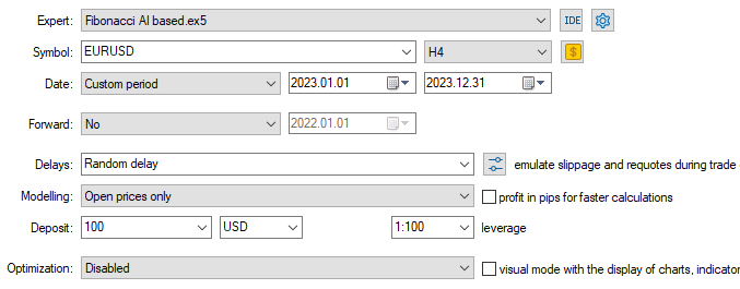
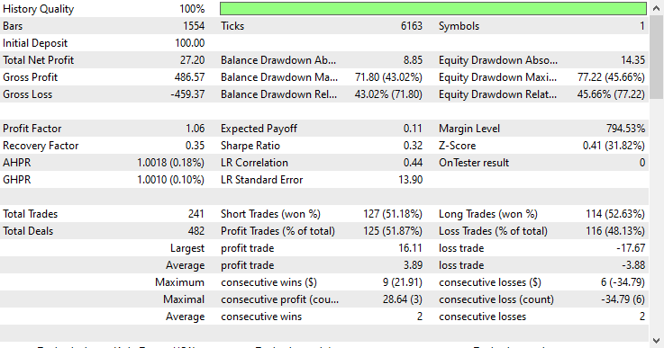
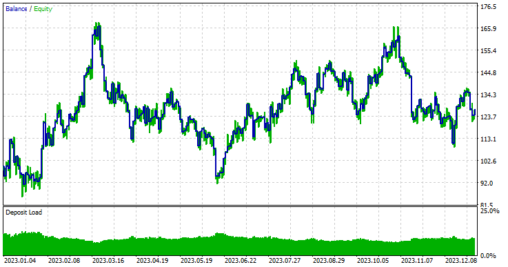
Model type: Classifier

Model type: Regressor

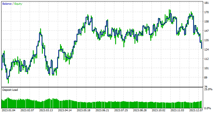
The regressor model did exceptionally well, considering this is the out-of-sample data, offering a 57.42% winning rate.

To make matters simple and a regressor model useful, inside the trading robot, I converted the continuous outcome provided by a random forest regressor model into a binary solution.

signal = pred_fib>iClose(Symbol(), Period(), 0)?1:0; //If the predicted Fibonacci is greater than the current close price, that's bullish otherwise that's bearish signal

This changes entirely the way we interpret the predicted Fibonacci level because, unlike what we usually do in manual trading where we open a trade at the end of the trend once we receive a trend confirmation signal or something. We set our trading targets to some Fibonacci level (usually 61.8%).

By using this approach, we assume that our machine learning models have already understood this pattern over a given lookback and lookahead window used on the training data so, we just to open some trades and hold them according to those specified number of bars.

The key here is the lookahead and the lookback window values, mainly because when we use the Fibonacci tool in manual trading, we don't consider the number of bars to use for its calculations (low and high values), we usually attach the tool where we see fit.

While the tool works fine in manual trading, it fools us into thinking we have the tool in the right place, when it's just us placing the tool where we want to place it without clear rules in mind.

These two values (lookahead and lookback windows) are the ones that we have to optimize if we are looking to explore the effectiveness of Fibonacci levels in creating the target variable and for machine learning usage in general.

Final Thoughts

Fibonacci retracements and levels are powerful techniques for creating the target variable for machine learning, as illustrated by the strategy tester report above produced by the regressor model. Even with as few predictors as Open, High, Low, and Close values, which don't offer many patterns, the models could detect some valuable patterns and make some good results compared to random guessing, based on the learned information from the Fibonacci levels.

No matter how you look at the outcomes, It's impressive in my opinion.

As it stands, this idea isn't polished enough, we need to add more features to our data such as indicator readings and some trading strategy confirmations to help our Fibonacci-based model capture complex patterns that happen in the market. Also, feel free to explore other fibonacci levels.

When this idea is improved further, I believe it will be much effective in the stock and indices markets where the pullbacks occur regularly in some bullish long-term trends, also in higher time frames like the daily timeframe where the data is "less noisy".

Attachments Table

Filename & Path	Description & Usage
Experts\Fibonacci AI based.mq5	The main expert advisor for testing machine learning models.
Include\Random Forest.mqh	Contains classes for loading and deploying the random forest classifier and regressor present in .ONNX format.
Files\*.onnx	Machine learning models in ONNX format.
Files\*.csv	CSV files containing datasets to be used for training machine learning models.
Python\fibbonanci-in-ml.ipynb	Python script for processing the data and training the random forest models.

Sources & References

Attached files |

Download ZIP

Attachments.zip (1525.28 KB)

Warning: All rights to these materials are reserved by MetaQuotes Ltd. Copying or reprinting of these materials in whole or in part is prohibited.

The Origin of Fibonacci Numbers

Understanding Fibonacci Retracement Levels from a Trading Aspect

Creating a Target Variable Using Fibonacci Retracements

Training a Classifier Model Based on the Fibonacci-Based Target Variable

Training a Regressor Model on the Fibonacci-Based Target Variable

Testing Fibonacci-Based Machine Learning Models on the Strategy Tester

Final Thoughts

Other articles by this author