How to use ONNX models in MQL5

Introduction

The authors of the article A CNN-LSTM-Based Model to Forecast Stock Prices (Wenjie Lu, Jiazheng Li, Yifan Li, Aijun Sun, Jingyang Wang, Complexity magazine, vol. 2020, Article ID 6622927, 10 pages, 2020) compared various stock prices forecasting models:

Stock price data have the characteristics of time series.

At the same time, based on machine learning long short-term memory (LSTM) which has the advantages of analyzing relationships among time series data through its memory function, we propose a forecasting method of stock price based on CNN-LSTM.

In the meanwhile, we use MLP, CNN, RNN, LSTM, CNN-RNN, and other forecasting models to predict the stock price one by one. Moreover, the forecasting results of these models are analyzed and compared. 
The data utilized in this research concern the daily stock prices from July 1, 1991, to August 31, 2020, including 7127 trading days.

In terms of historical data, we choose eight features, including opening price, highest price, lowest price, closing price, volume, turnover, ups and downs, and change. 
Firstly, we adopt CNN to efficiently extract features from the data, which are the items of the previous 10 days. And then, we adopt LSTM to predict the stock price with the extracted feature data.

According to the experimental results, the CNN-LSTM can provide a reliable stock price forecasting with the highest prediction accuracy.
This forecasting method not only provides a new research idea for stock price forecasting but also provides practical experience for scholars to study financial time series data.

Among all the considered models, CNN-LSTM models have generated the best results during the experiments. In this article, we will consider how to create such a model to forecast financial timeseries and how to use the created ONNX model in an MQL5 Expert Advisor.

1. Building a model

Python offers a set of specialized libraries and thus it provides extensive capabilities for working with ML models. Libraries greatly facilitate data preparation and processing.

We recommend using GPU resources to maximize the efficiency of ML projects. Many Windows users encountered problems trying to install the current TensorFlow version (See comments on the video guide and its text version). So, we have tested TensorFlow 2.10.0 and recommend using this version. GPU computations were performed on NVIDIA GeForce RTX 2080 Ti graphics card using CUDA 11.2 and CUDNN 8.1.0.7 libraries.

1.1. Installing Python and libraries

If you do not have Python, you should install it. We used version 3.9.16.

Also, install the libraries (If you are using Conda/Anaconda, run these commands in Anaconda Prompt):

python.exe -m pip install --upgrade pip
pip install --upgrade pandas
pip install --upgrade scikit-learn
pip install --upgrade matplotlib
pip install --upgrade tqdm
pip install --upgrade metatrader5
pip install --upgrade onnx==1.12
pip install --upgrade tf2onnx
pip install --upgrade tensorflow==2.10.0

1.2. Checking TensorFlow version and GPU

The below code checks the installed TensorFlow version and verifies whether it is possible to use the GPU to compute the models:

#check tensorflow version
print(tf.__version__)
#check GPU support
print(len(tf.config.list_physical_devices('GPU'))>0)

If the required version is installed correctly, you will see the following result:

2.10.0
True

We used a Python script to build and train the model. The steps of this process are briefly described below.

1.3. Building and training the model

The script starts by importing the Python libraries which will be used in the model.

#Python libraries
import matplotlib.pyplot as plt 
import MetaTrader5 as mt5
import tensorflow as tf
import numpy as np
import pandas as pd
import tf2onnx
from sklearn.model_selection import train_test_split
from sys import argv

Check TensorFlow version and GPU availability:

#check tensorflow version
print(tf.__version__)

2.10.0

#check GPU support
print(len(tf.config.list_physical_devices('GPU'))>0)

True

Initialize MetaTrader 5 for operations from Python:

#initialize MetaTrader5 for history data
if not mt5.initialize():
    print("initialize() failed, error code =",mt5.last_error())
    quit()

Information about the MetaTrader 5 terminal:

#show terminal info
terminal_info=mt5.terminal_info()
print(terminal_info)

TerminalInfo(community_account=True, community_connection=True, connected=True, dlls_allowed=False, trade_allowed=False, tradeapi_disabled=False, email_enabled=False, ftp_enabled=False, notifications_enabled=False, mqid=False, build=3640, maxbars=100000, codepage=0, ping_last=58768, community_balance=1.0, retransmission=0.015296317559440137, company='MetaQuotes Software Corp.', name='MetaTrader 5', language='English', path='C:\\Program Files\\MetaTrader 5', data_path='C:\\Users\\user\\AppData\\Roaming\\MetaQuotes\\Terminal\\D0E8209F77C8CF37AD8BF550E51FF075', commondata_path='C:\\Users\\user\\AppData\\Roaming\\MetaQuotes\\Terminal\\Common')

#show file path
file_path=terminal_info.data_path+"\\MQL5\\Files\\"
print(file_path)

C:\Users\user\AppData\Roaming\MetaQuotes\Terminal\D0E8209F77C8CF37AD8BF550E51FF075\MQL5\Files\

Print the path to save the model (in this example, the script runs in Jupyter Notebook):

#data path to save the model
data_path=argv[0]
last_index=data_path.rfind("\\")+1
data_path=data_path[0:last_index]
print("data path to save onnx model",data_path)

data path to save onnx model C:\Users\user\AppData\Roaming\Python\Python39\site-packages\

Prepare dates to request historical data. In our example, we request EURUSD H1 bars for 120 from the current date:

#set start and end dates for history data
from datetime import timedelta,datetime
end_date = datetime.now()
start_date = end_date - timedelta(days=120)

#print start and end dates
print("data start date=",start_date)
print("data end date=",end_date)

data start date= 2022-11-28 12:28:39.870685
data end date= 2023-03-28 12:28:39.870685

Request EURUSD historical data:

#get EURUSD rates (H1) from start_date to end_date
eurusd_rates = mt5.copy_rates_range("EURUSD", mt5.TIMEFRAME_H1, start_date, end_date)

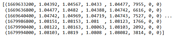
Output the downloaded data:

#check
print(eurusd_rates)

#create dataframe
df = pd.DataFrame(eurusd_rates)

Show the dataframe beginning and end:

#show dataframe head
df.head()

#show dataframe tail
df.tail()

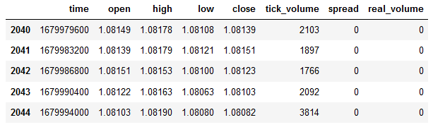
#show dataframe shape (the number of rows and columns in the data set)
df.shape

(2045, 8)

Select Close prices only:

#prepare close prices only
data = df.filter(['close']).values

Output the data:

#show close prices
plt.figure(figsize = (18,10))
plt.plot(data,'b',label = 'Original')
plt.xlabel("Hours")
plt.ylabel("Price")
plt.title("EURUSD_H1")
plt.legend()

Scale the source price data to the range [0,1] using MinMaxScaler:

#scale data using MinMaxScaler
from sklearn.preprocessing import MinMaxScaler
scaler=MinMaxScaler(feature_range=(0,1))
scaled_data = scaler.fit_transform(data)

The first 80% of the data will be used for training.

#training size is 80% of the data
training_size = int(len(scaled_data)*0.80) 
print("training size:",training_size)

training size: 1636

#create train data and check size
train_data_initial = scaled_data[0:training_size,:]
print(len(train_data_initial))

1636

#create test data and check size
test_data_initial= scaled_data[training_size:,:1]
print(len(test_data_initial))

409

The following function creates training sequences:

#split a univariate sequence into samples
def split_sequence(sequence, n_steps):
    X, y = list(), list()
    for i in range(len(sequence)):
       #find the end of this pattern
       end_ix = i + n_steps
       #check if we are beyond the sequence
       if end_ix > len(sequence)-1:
          break
       #gather input and output parts of the pattern
       seq_x, seq_y = sequence[i:end_ix], sequence[end_ix]
       X.append(seq_x)
       y.append(seq_y)
    return np.array(X), np.array(y)

Build the sets:

#split into samples
time_step = 120
x_train, y_train = split_sequence(train_data_initial, time_step)
x_test, y_test = split_sequence(test_data_initial, time_step)
#reshape input to be [samples, time steps, features] which is required for LSTM
x_train =x_train.reshape(x_train.shape[0],x_train.shape[1],1)
x_test = x_test.reshape(x_test.shape[0],x_test.shape[1],1)

Tensor shapes for training and testing:

#show shape of train data
x_train.shape

(1516, 120, 1)

#show shape of test data
x_test.shape

(289, 120, 1)

#import keras libraries for the model
import math
from keras.models import Sequential
from keras.layers import Dense,Activation,Conv1D,MaxPooling1D,Dropout
from keras.layers import LSTM
from keras.utils.vis_utils import plot_model
from keras.metrics import RootMeanSquaredError as rmse
from keras import optimizers

Set the model:

#define the model
model = Sequential()
model.add(Conv1D(filters=256, kernel_size=2,activation='relu',padding = 'same',input_shape=(120,1)))
model.add(MaxPooling1D(pool_size=2))
model.add(LSTM(100, return_sequences = True))
model.add(Dropout(0.3))
model.add(LSTM(100, return_sequences = False))
model.add(Dropout(0.3))
model.add(Dense(units=1, activation = 'sigmoid'))
model.compile(optimizer='adam', loss= 'mse' , metrics = [rmse()])

Show the model properties:

#show model
model.summary()

Model training:

#measure time
import time 
time_calc_start = time.time()

#fit model with 300 epochs
history=model.fit(x_train,y_train,epochs=300,validation_data=(x_test,y_test),batch_size=32,verbose=1)

#calculate time
fit_time_seconds = time.time() - time_calc_start
print("fit time =",fit_time_seconds," seconds.")

Epoch 1/300
48/48 [==============================] - 8s 49ms/step - loss: 0.0129 - root_mean_squared_error: 0.1136 - val_loss: 0.0065 - val_root_mean_squared_error: 0.0804

...

Epoch 299/300
48/48 [==============================] - 2s 35ms/step - loss: 4.5197e-04 - root_mean_squared_error: 0.0213 - val_loss: 4.2535e-04 - val_root_mean_squared_error: 0.0206
Epoch 300/300
48/48 [==============================] - 2s 32ms/step - loss: 4.2967e-04 - root_mean_squared_error: 0.0207 - val_loss: 4.4040e-04 - val_root_mean_squared_error: 0.0210

fit time = 467.4918096065521  seconds.

The training took about 8 minutes.

#show training history keys
history.history.keys()

dict_keys(['loss', 'root_mean_squared_error', 'val_loss', 'val_root_mean_squared_error'])

Optimization dynamics in the training and testing datasets:

#show iteration-loss graph for training and validation
plt.figure(figsize = (18,10))
plt.plot(history.history['loss'],label='Training Loss',color='b')
plt.plot(history.history['val_loss'],label='Validation-loss',color='g')
plt.xlabel("Iteration")
plt.ylabel("Loss")
plt.title("LOSS")
plt.legend()

#show iteration-rmse graph for training and validation
plt.figure(figsize = (18,10))
plt.plot(history.history['root_mean_squared_error'],label='Training RMSE',color='b')
plt.plot(history.history['val_root_mean_squared_error'],label='Validation-RMSE',color='g')
plt.xlabel("Iteration")
plt.ylabel("RMSE")
plt.title("RMSE")
plt.legend()

#evaluate training data
model.evaluate(x_train,y_train, batch_size = 32)

48/48 [==============================] - 1s 22ms/step - loss: 2.9911e-04 - root_mean_squared_error: 0.0173
[0.00029911252204328775, 0.01729486882686615]

#evaluate testing data
model.evaluate(x_test,y_test, batch_size = 32)

10/10 [==============================] - 0s 31ms/step - loss: 4.4040e-04 - root_mean_squared_error: 0.0210

[0.00044039846397936344, 0.020985672250390053]

Forming the prediction on the training dataset:

#prediction using training data
train_predict = model.predict(x_train)
plot_y_train = y_train.reshape(-1,1)

48/48 [==============================] - 2s 18ms/step

Output actual and predicted graphs for the training interval:

#show actual vs predicted (training) graph
plt.figure(figsize=(18,10))
plt.plot(scaler.inverse_transform(plot_y_train),color = 'b', label = 'Original')
plt.plot(scaler.inverse_transform(train_predict),color='red', label = 'Predicted')
plt.title("Prediction Graph Using Training Data")
plt.xlabel("Hours")
plt.ylabel("Price")
plt.legend()
plt.show()

Forming the prediction on the testing dataset:

#prediction using testing data
test_predict = model.predict(x_test)
plot_y_test = y_test.reshape(-1,1)

11/11 [==============================] - 0s 11ms/step

To calculate metrics, we need to convert the data from the interval [0,1]. Again, we use MinMaxScaler.

#calculate metrics
from sklearn import metrics
from sklearn.metrics import r2_score
#transform data to real values
value1=scaler.inverse_transform(plot_y_test)
value2=scaler.inverse_transform(test_predict)
#calc score
score = np.sqrt(metrics.mean_squared_error(value1,value2))
print("RMSE         : {}".format(score))
print("MSE          :", metrics.mean_squared_error(value1,value2))
print("R2 score     :",metrics.r2_score(value1,value2))

RMSE         : 0.0015151631684117558
MSE          : 2.295719426911551e-06
R2 score     : 0.9683533377809039

#show actual vs predicted (testing) graph
plt.figure(figsize=(18,10))
plt.plot(scaler.inverse_transform(plot_y_test),color = 'b',  label = 'Original')
plt.plot(scaler.inverse_transform(test_predict),color='g', label = 'Predicted')
plt.title("Prediction Graph Using Testing Data")
plt.xlabel("Hours")
plt.ylabel("Price")
plt.legend()
plt.show()

Export the model to an onnx file:

# save model to ONNX
output_path = data_path+"model.eurusd.H1.120.onnx"
onnx_model = tf2onnx.convert.from_keras(model, output_path=output_path)
print(f"model saved to {output_path}")

output_path = file_path+"model.eurusd.H1.120.onnx"
onnx_model = tf2onnx.convert.from_keras(model, output_path=output_path)
print(f"saved model to {output_path}")

# finish
mt5.shutdown()

The full code of the Python script is attached to the article in a Jupyter Notebook.

In the article A CNN-LSTM-Based Model to Forecast Stock Prices, the best result R^2=0.9646 was obtained for models with the CNN-LSTM architecture. In our example, the CNN-LSTM network has generated the best result of R^2=0.9684. According to the results, models of this type can be efficient in solving prediction problems.

We have considered an example of a Python script which builds and trains CNN-LSTM models to predict financial timeseries.

2. Using the Model in MetaTrader 5

2.1. Good to know before you get started

There are two ways to create a model: You can use OnnxCreate to create a model from an onnx file or OnnxCreateFromBuffer to create it from a data array.

If an ONNX model is used as a resources in an EA, you will need to recompile the EA every time you change the model.

Not all models have fully defined sizes input and/or output tensor. This is normally the first dimension responsible for the package size. Before running a model, you must explicitly specify the sizes using the OnnxSetInputShape and OnnxSetOutputShape functions. The model's input data should be prepared in the same way as it was done when training the model.

For input and output data, we recommend using the arrays, matrices and/or vectors of the same type that are used in the model. In this case, you will not have to convert data when running the model. If the data cannot be represented in the required type, the data will be automatically converted.

Use the OnnxRun to inference (run) your model. Note that a model can be run multiple times. After using the model, release it using the OnnxRelease function.

Complete documentation for ONNX models in MQL5.

2.2. Reading an onnx file and getting information on inputs and outputs

In order to use our model, we need to know the model location, input data type and shape, as well as output data type and shape. According to the previously created script, model.eurusd.H1.120.onnx is located in the same folder with the Python script that has generated the onnx file. Input is float32, 120 normalized Close prices (for working with the batch size equal to 1); output is float32, which is one normalized price predicted by the model.

We have also created the onnx file in the MQL5\Files folder in order to obtain the model input and output data using an MQL5 script.

//+------------------------------------------------------------------+
//|                                                OnnxModelInfo.mq5 |
//|                                  Copyright 2023, MetaQuotes Ltd. |
//|                                             https://www.mql5.com |
//+------------------------------------------------------------------+
#property copyright "Copyright 2023, MetaQuotes Ltd."
#property link      "https://www.mql5.com"
#property version   "1.00"

#define UNDEFINED_REPLACE 1

//+------------------------------------------------------------------+
//| Script program start function                                    |
//+------------------------------------------------------------------+
void OnStart()
  {
   string file_names[];
   if(FileSelectDialog("Open ONNX model",NULL,"ONNX files (*.onnx)|*.onnx|All files (*.*)|*.*",FSD_FILE_MUST_EXIST,file_names,NULL)<1)
      return;

   PrintFormat("Create model from %s with debug logs",file_names[0]);

   long session_handle=OnnxCreate(file_names[0],ONNX_DEBUG_LOGS);
   if(session_handle==INVALID_HANDLE)
     {
      Print("OnnxCreate error ",GetLastError());
      return;
     }

   OnnxTypeInfo type_info;

   long input_count=OnnxGetInputCount(session_handle);
   Print("model has ",input_count," input(s)");
   for(long i=0; i<input_count; i++)
     {
      string input_name=OnnxGetInputName(session_handle,i);
      Print(i," input name is ",input_name);
      if(OnnxGetInputTypeInfo(session_handle,i,type_info))
         PrintTypeInfo(i,"input",type_info);
     }

   long output_count=OnnxGetOutputCount(session_handle);
   Print("model has ",output_count," output(s)");
   for(long i=0; i<output_count; i++)
     {
      string output_name=OnnxGetOutputName(session_handle,i);
      Print(i," output name is ",output_name);
      if(OnnxGetOutputTypeInfo(session_handle,i,type_info))
         PrintTypeInfo(i,"output",type_info);
     }

   OnnxRelease(session_handle);
  }
//+------------------------------------------------------------------+
//| PrintTypeInfo                                                    |
//+------------------------------------------------------------------+
void PrintTypeInfo(const long num,const string layer,const OnnxTypeInfo& type_info)
  {
   Print("   type ",EnumToString(type_info.type));
   Print("   data type ",EnumToString(type_info.element_type));

   if(type_info.dimensions.Size()>0)
     {
      bool   dim_defined=(type_info.dimensions[0]>0);
      string dimensions=IntegerToString(type_info.dimensions[0]);
      for(long n=1; n<type_info.dimensions.Size(); n++)
        {
         if(type_info.dimensions[n]<=0)
            dim_defined=false;
         dimensions+=", ";
         dimensions+=IntegerToString(type_info.dimensions[n]);
        }
      Print("   shape [",dimensions,"]");
      //--- not all dimensions defined
      if(!dim_defined)
         PrintFormat("   %I64d %s shape must be defined explicitly before model inference",num,layer);
      //--- reduce shape
      uint reduced=0;
      long dims[];
      for(long n=0; n<type_info.dimensions.Size(); n++)
        {
         long dimension=type_info.dimensions[n];
         //--- replace undefined dimension
         if(dimension<=0)
            dimension=UNDEFINED_REPLACE;
         //--- 1 can be reduced
         if(dimension>1)
           {
            ArrayResize(dims,reduced+1);
            dims[reduced++]=dimension;
           }
        }
      //--- all dimensions assumed 1
      if(reduced==0)
        {
         ArrayResize(dims,1);
         dims[reduced++]=1;
        }
      //--- shape was reduced
      if(reduced<type_info.dimensions.Size())
        {
         dimensions=IntegerToString(dims[0]);
         for(long n=1; n<dims.Size(); n++)
           {
            dimensions+=", ";
            dimensions+=IntegerToString(dims[n]);
           }
         string sentence="";
         if(!dim_defined)
            sentence=" if undefined dimension set to "+(string)UNDEFINED_REPLACE;
         PrintFormat("   shape of %s data can be reduced to [%s]%s",layer,dimensions,sentence);
        }
     }
   else
      PrintFormat("no dimensions defined for %I64d %s",num,layer);
  }
//+------------------------------------------------------------------+

In the file selection window, we selected the onnx file saved in MQL5\Files, created a model from the file using OnnxCreate and obtained the following information.

Create model from model.eurusd.H1.120.onnx with debug logs
ONNX: Creating and using per session threadpools since use_per_session_threads_ is true
ONNX: Dynamic block base set to 0
ONNX: Initializing session.
ONNX: Adding default CPU execution provider.
ONNX: Total shared scalar initializer count: 0
ONNX: Total fused reshape node count: 0
ONNX: Removing NodeArg 'Gather_out0'. It is no longer used by any node.
ONNX: Removing NodeArg 'Gather_token_1_out0'. It is no longer used by any node.
ONNX: Total shared scalar initializer count: 0
ONNX: Total fused reshape node count: 0
ONNX: Removing initializer 'sequential/conv1d/Conv1D/ExpandDims_1:0'. It is no longer used by any node.
ONNX: Use DeviceBasedPartition as default
ONNX: Saving initialized tensors.
ONNX: Done saving initialized tensors
ONNX: Session successfully initialized.
model has 1 input(s)
0 input name is conv1d_input
   type ONNX_TYPE_TENSOR
   data type ONNX_DATA_TYPE_FLOAT
   shape [-1, 120, 1]
   0 input shape must be defined explicitly before model inference
   shape of input data can be reduced to [120] if undefined dimension set to 1
model has 1 output(s)
0 output name is dense
   type ONNX_TYPE_TENSOR
   data type ONNX_DATA_TYPE_FLOAT
   shape [-1, 1]
   0 output shape must be defined explicitly before model inference
   shape of output data can be reduced to [1] if undefined dimension set to 1

Since the debugging mode was enabled

   long session_handle=OnnxCreate(file_names[0],ONNX_DEBUG_LOGS);

we have logs with the ONNX prefix.

We see that the model actually has one input and one output. Here, the first dimension of the input tensor and the first dimension of the output tensor are not defined. It is assumed that these dimensions are responsible for the batch size. Therefore, before inferencing the model, we must explicitly specify what sizes we are going to work with (OnnxSetInputShape and OnnxSetOutputShape). Usually only one dataset is input into the model. A detailed example is provided in the next paragraph "An example of using an ONNX model in a trading EA".

When preparing the data, it is not necessary to use an array with dimensions [1, 120, 1]. We can input a one-dimensional array or a 120-element vector.

2.3. An example of using an ONNX model in a trading EA

Declarations and definitions

#include <Trade\Trade.mqh>

input double InpLots = 1.0;    // Lots amount to open position

#resource "Python/model.120.H1.onnx" as uchar ExtModel[]

#define SAMPLE_SIZE 120

long     ExtHandle=INVALID_HANDLE;
int      ExtPredictedClass=-1;
datetime ExtNextBar=0;
datetime ExtNextDay=0;
float    ExtMin=0.0;
float    ExtMax=0.0;
CTrade   ExtTrade;

//--- price movement prediction
#define PRICE_UP   0
#define PRICE_SAME 1
#define PRICE_DOWN 2

OnInit function

//+------------------------------------------------------------------+
//| Expert initialization function                                   |
//+------------------------------------------------------------------+
int OnInit()
  {
   if(_Symbol!="EURUSD" || _Period!=PERIOD_H1)
     {
      Print("model must work with EURUSD,H1");
      return(INIT_FAILED);
     }

//--- create a model from static buffer
   ExtHandle=OnnxCreateFromBuffer(ExtModel,ONNX_DEFAULT);
   if(ExtHandle==INVALID_HANDLE)
     {
      Print("OnnxCreateFromBuffer error ",GetLastError());
      return(INIT_FAILED);
     }

//--- since not all sizes defined in the input tensor we must set them explicitly
//--- first index - batch size, second index - series size, third index - number of series (only Close)
   const long input_shape[] = {1,SAMPLE_SIZE,1};
   if(!OnnxSetInputShape(ExtHandle,ONNX_DEFAULT,input_shape))
     {
      Print("OnnxSetInputShape error ",GetLastError());
      return(INIT_FAILED);
     }

//--- since not all sizes defined in the output tensor we must set them explicitly
//--- first index - batch size, must match the batch size of the input tensor
//--- second index - number of predicted prices (we only predict Close)
   const long output_shape[] = {1,1};
   if(!OnnxSetOutputShape(ExtHandle,0,output_shape))
     {
      Print("OnnxSetOutputShape error ",GetLastError());
      return(INIT_FAILED);
     }
//---
   return(INIT_SUCCEEDED);
  }

We only work with EURUSD, H1, because we use the current symbol/period data.

Our model is included in the EA as a resource. The EA is completely self-sufficient and does not require to read an external onnx file. A model is created from the resource array.

The input and output data shapes must be explicitly defined.

The OnTick function:

//+------------------------------------------------------------------+
//| Expert tick function                                             |
//+------------------------------------------------------------------+
void OnTick()
  {
//--- check new day
   if(TimeCurrent()>=ExtNextDay)
     {
      GetMinMax();
      //--- set next day time
      ExtNextDay=TimeCurrent();
      ExtNextDay-=ExtNextDay%PeriodSeconds(PERIOD_D1);
      ExtNextDay+=PeriodSeconds(PERIOD_D1);
     }

//--- check new bar
   if(TimeCurrent()<ExtNextBar)
      return;
//--- set next bar time
   ExtNextBar=TimeCurrent();
   ExtNextBar-=ExtNextBar%PeriodSeconds();
   ExtNextBar+=PeriodSeconds();
//--- check min and max
   double close=iClose(_Symbol,_Period,0);
   if(ExtMin>close)
      ExtMin=close;
   if(ExtMax<close)
      ExtMax=close;

//--- predict next price
   PredictPrice();
//--- check trading according to prediction
   if(ExtPredictedClass>=0)
      if(PositionSelect(_Symbol))
         CheckForClose();
      else
         CheckForOpen();
  }

We define the beginning of a new day. The day beginning is used to update the Low and High values of the 120-day sequence to normalize prices in the 120-hour sequence. The model was trained under these conditions, which we must follow when preparing input data.

//+------------------------------------------------------------------+
//| Get minimal and maximal Close for last 120 days                  |
//+------------------------------------------------------------------+
void GetMinMax(void)
  {
   vectorf close;
   close.CopyRates(_Symbol,PERIOD_D1,COPY_RATES_CLOSE,0,SAMPLE_SIZE);
   ExtMin=close.Min();
   ExtMax=close.Max();
  }

If necessary, we can modify Low and High throughout the day.

Prediction function:

//+------------------------------------------------------------------+
//| Predict next price                                               |
//+------------------------------------------------------------------+
void PredictPrice(void)
  {
   static vectorf output_data(1);            // vector to get result
   static vectorf x_norm(SAMPLE_SIZE);       // vector for prices normalize

//--- check for normalization possibility
   if(ExtMin>=ExtMax)
     {
      ExtPredictedClass=-1;
      return;
     }
//--- request last bars
   if(!x_norm.CopyRates(_Symbol,_Period,COPY_RATES_CLOSE,1,SAMPLE_SIZE))
     {
      ExtPredictedClass=-1;
      return;
     }
   float last_close=x_norm[SAMPLE_SIZE-1];
//--- normalize prices
   x_norm-=ExtMin;
   x_norm/=(ExtMax-ExtMin);
//--- run the inference
   if(!OnnxRun(ExtHandle,ONNX_NO_CONVERSION,x_norm,output_data))
     {
      ExtPredictedClass=-1;
      return;
     }
//--- denormalize the price from the output value
   float predicted=output_data[0]*(ExtMax-ExtMin)+ExtMin;
//--- classify predicted price movement
   float delta=last_close-predicted;
   if(fabs(delta)<=0.00001)
      ExtPredictedClass=PRICE_SAME;
   else
     {
      if(delta<0)
         ExtPredictedClass=PRICE_UP;
      else
         ExtPredictedClass=PRICE_DOWN;
     }
  }

First, we check if we can normalize. Normalization is implemented as in the MinMaxScaler Python function.

#scale data
from sklearn.preprocessing import MinMaxScaler
scaler=MinMaxScaler(feature_range=(0,1))
scaled_data = scaler.fit_transform(data)

So, the normalization code is very simple and straightforward.

The vectors for input data and for receiving the result are organized as static. This guarantees a non-relocatable buffer that exists for the entire program lifetime. Thus, the ONNX model's input and output tensors are not recreated each time we run the model.

The key function is OnnxRun. The ONNX_NO_CONVERSION flag indicates that the input and output data must not be converted since the MQL5 float type exactly corresponds to ONNX_DATA_TYPE_FLOAT. The ONNX_DEBUG flag is not set.

After that, we denormalize the obtained data into the predicted price and determine the class: whether the price will go up, down, or will not change.

The trading strategy is simple. At the beginning of each hour, we check the price forecast for the end of that hour. If the predicted price goes up, we buy. If the model predicts a down movement, we sell.

//+------------------------------------------------------------------+
//| Check for open position conditions                               |
//+------------------------------------------------------------------+
void CheckForOpen(void)
  {
   ENUM_ORDER_TYPE signal=WRONG_VALUE;
//--- check signals
   if(ExtPredictedClass==PRICE_DOWN)
      signal=ORDER_TYPE_SELL;    // sell condition
   else
     {
      if(ExtPredictedClass==PRICE_UP)
         signal=ORDER_TYPE_BUY;  // buy condition
     }

//--- open position if possible according to signal
   if(signal!=WRONG_VALUE && TerminalInfoInteger(TERMINAL_TRADE_ALLOWED))
     {
      double price;
      double bid=SymbolInfoDouble(_Symbol,SYMBOL_BID);
      double ask=SymbolInfoDouble(_Symbol,SYMBOL_ASK);
      if(signal==ORDER_TYPE_SELL)
         price=bid;
      else
         price=ask;
      ExtTrade.PositionOpen(_Symbol,signal,InpLots,price,0.0,0.0);
     }
  }
//+------------------------------------------------------------------+
//| Check for close position conditions                              |
//+------------------------------------------------------------------+
void CheckForClose(void)
  {
   bool bsignal=false;
//--- position already selected before
   long type=PositionGetInteger(POSITION_TYPE);
//--- check signals
   if(type==POSITION_TYPE_BUY && ExtPredictedClass==PRICE_DOWN)
      bsignal=true;
   if(type==POSITION_TYPE_SELL && ExtPredictedClass==PRICE_UP)
      bsignal=true;

//--- close position if possible
   if(bsignal && TerminalInfoInteger(TERMINAL_TRADE_ALLOWED))
     {
      ExtTrade.PositionClose(_Symbol,3);
      //--- open opposite
      CheckForOpen();
     }
  }

Now, let us check the EA performance in the Strategy Tester. In order to test the EA from the beginning of the year, the model should be trained using earlier data. Therefore, we slightly modified the Python script by removing unused parts and changing the training end date so that it does not overlap with the testing period.

The ONNX.eurusd.H1.120.Training.py script is located in the Python subfolder and runs directly in MetaEditor. The resulting ONNX model will be saved in the same Python subfolder and will be used as a resource during the EA compilation.

# Copyright 2023, MetaQuotes Ltd.
# https://www.mql5.com

# python libraries
import MetaTrader5 as mt5
import tensorflow as tf
import numpy as np
import pandas as pd
import tf2onnx

# input parameters
inp_model_name = "model.eurusd.H1.120.onnx"
inp_history_size = 120

if not mt5.initialize():
    print("initialize() failed, error code =",mt5.last_error())
    quit()

# we will save generated onnx-file near our script to use as resource
from sys import argv
data_path=argv[0]
last_index=data_path.rfind("\\")+1
data_path=data_path[0:last_index]
print("data path to save onnx model",data_path)

# set start and end dates for history data
from datetime import timedelta, datetime
#end_date = datetime.now()
end_date = datetime(2023, 1, 1, 0)
start_date = end_date - timedelta(days=inp_history_size)

# print start and end dates
print("data start date =",start_date)
print("data end date =",end_date)

# get rates
eurusd_rates = mt5.copy_rates_range("EURUSD", mt5.TIMEFRAME_H1, start_date, end_date)

# create dataframe
df = pd.DataFrame(eurusd_rates)

# get close prices only
data = df.filter(['close']).values

# scale data
from sklearn.preprocessing import MinMaxScaler
scaler=MinMaxScaler(feature_range=(0,1))
scaled_data = scaler.fit_transform(data)

# training size is 80% of the data
training_size = int(len(scaled_data)*0.80) 
print("Training_size:",training_size)
train_data_initial = scaled_data[0:training_size,:]
test_data_initial = scaled_data[training_size:,:1]

# split a univariate sequence into samples
def split_sequence(sequence, n_steps):
    X, y = list(), list()
    for i in range(len(sequence)):
       # find the end of this pattern
       end_ix = i + n_steps
       # check if we are beyond the sequence
       if end_ix > len(sequence)-1:
          break
       # gather input and output parts of the pattern
       seq_x, seq_y = sequence[i:end_ix], sequence[end_ix]
       X.append(seq_x)
       y.append(seq_y)
    return np.array(X), np.array(y)

# split into samples
time_step = inp_history_size
x_train, y_train = split_sequence(train_data_initial, time_step)
x_test, y_test = split_sequence(test_data_initial, time_step)

# reshape input to be [samples, time steps, features] which is required for LSTM
x_train =x_train.reshape(x_train.shape[0],x_train.shape[1],1)
x_test = x_test.reshape(x_test.shape[0],x_test.shape[1],1)

# define model
from keras.models import Sequential
from keras.layers import Dense, Activation, Conv1D, MaxPooling1D, Dropout, Flatten, LSTM
from keras.metrics import RootMeanSquaredError as rmse
model = Sequential()
model.add(Conv1D(filters=256, kernel_size=2, activation='relu',padding = 'same',input_shape=(inp_history_size,1)))
model.add(MaxPooling1D(pool_size=2))
model.add(LSTM(100, return_sequences = True))
model.add(Dropout(0.3))
model.add(LSTM(100, return_sequences = False))
model.add(Dropout(0.3))
model.add(Dense(units=1, activation = 'sigmoid'))
model.compile(optimizer='adam', loss= 'mse' , metrics = [rmse()])

# model training for 300 epochs
history = model.fit(x_train, y_train, epochs = 300 , validation_data = (x_test,y_test), batch_size=32, verbose=2)

# evaluate training data
train_loss, train_rmse = model.evaluate(x_train,y_train, batch_size = 32)
print(f"train_loss={train_loss:.3f}")
print(f"train_rmse={train_rmse:.3f}")

# evaluate testing data
test_loss, test_rmse = model.evaluate(x_test,y_test, batch_size = 32)
print(f"test_loss={test_loss:.3f}")
print(f"test_rmse={test_rmse:.3f}")

# save model to ONNX
output_path = data_path+inp_model_name
onnx_model = tf2onnx.convert.from_keras(model, output_path=output_path)
print(f"saved model to {output_path}")

# finish
mt5.shutdown()

Testing an ONNX model based EA

Now, let us test the EA on historical data in the Strategy Tester. We specify the same parameters that we used to train the model: the EURUSD symbol and the H1 timeframe.

The testing interval does not include the training period: it starts from the beginning of the year (01/01/2023). 

According to the strategy, the signals are checked once, at the beginning of each hour (the EA monitors the emergence of a new bar), therefore, the tick modeling mode does not matter. OnTick will be processed in the tester once per bar.

//+------------------------------------------------------------------+
//| Expert tick function                                             |
//+------------------------------------------------------------------+
void OnTick()
  {
//--- check new day
   if(TimeCurrent()>=ExtNextDay)
     {
      GetMinMax();
      //--- set next day time
      ExtNextDay=TimeCurrent();
      ExtNextDay-=ExtNextDay%PeriodSeconds(PERIOD_D1);
      ExtNextDay+=PeriodSeconds(PERIOD_D1);
     }

//--- check new bar
   if(TimeCurrent()<ExtNextBar)
      return;
//--- set next bar time
   ExtNextBar=TimeCurrent();
   ExtNextBar-=ExtNextBar%PeriodSeconds();
   ExtNextBar+=PeriodSeconds();
//--- check min and max
   float close=(float)iClose(_Symbol,_Period,0);
   if(ExtMin>close)
      ExtMin=close;
   if(ExtMax<close)
      ExtMax=close;

//--- predict next price
   PredictPrice();
//--- check trading according to prediction
   if(ExtPredictedClass>=0)
      if(PositionSelect(_Symbol))
         CheckForClose();
      else
         CheckForOpen();
  }

With this processing, the three-month period testing takes only a few seconds. Below are the results.

Now, let us modify the trading strategy to enable position opening by a signal and closing by Stop Loss (SL) or Take Profit (TP).

input double InpLots       = 1.0;    // Lots amount to open position
input bool   InpUseStops   = true;   // Use stops in trading
input int    InpTakeProfit = 500;    // TakeProfit level
input int    InpStopLoss   = 500;    // StopLoss level

//+------------------------------------------------------------------+
//| Check for open position conditions                               |
//+------------------------------------------------------------------+
void CheckForOpen(void)
  {
   ENUM_ORDER_TYPE signal=WRONG_VALUE;
//--- check signals
   if(ExtPredictedClass==PRICE_DOWN)
      signal=ORDER_TYPE_SELL;    // sell condition
   else
     {
      if(ExtPredictedClass==PRICE_UP)
         signal=ORDER_TYPE_BUY;  // buy condition
     }

//--- open position if possible according to signal
   if(signal!=WRONG_VALUE && TerminalInfoInteger(TERMINAL_TRADE_ALLOWED))
     {
      double price,sl=0,tp=0;
      double bid=SymbolInfoDouble(_Symbol,SYMBOL_BID);
      double ask=SymbolInfoDouble(_Symbol,SYMBOL_ASK);
      if(signal==ORDER_TYPE_SELL)
        {
         price=bid;
         if(InpUseStops)
           {
            sl=NormalizeDouble(bid+InpStopLoss*_Point,_Digits);
            tp=NormalizeDouble(ask-InpTakeProfit*_Point,_Digits);
           }
        }
      else
        {
         price=ask;
         if(InpUseStops)
           {
            sl=NormalizeDouble(ask-InpStopLoss*_Point,_Digits);
            tp=NormalizeDouble(bid+InpTakeProfit*_Point,_Digits);
           }
        }
      ExtTrade.PositionOpen(_Symbol,signal,InpLots,price,sl,tp);
     }
  }
//+------------------------------------------------------------------+
//| Check for close position conditions                              |
//+------------------------------------------------------------------+
void CheckForClose(void)
  {
//--- position should be closed by stops
   if(InpUseStops)
      return;

   bool bsignal=false;
//--- position already selected before
   long type=PositionGetInteger(POSITION_TYPE);
//--- check signals
   if(type==POSITION_TYPE_BUY && ExtPredictedClass==PRICE_DOWN)
      bsignal=true;
   if(type==POSITION_TYPE_SELL && ExtPredictedClass==PRICE_UP)
      bsignal=true;

//--- close position if possible
   if(bsignal && TerminalInfoInteger(TERMINAL_TRADE_ALLOWED))
     {
      ExtTrade.PositionClose(_Symbol,3);
      //--- open opposite
      CheckForOpen();
     }
  }

InpUseStops = true, which means that SL and TP levels are set at position opening.

The results of testing with SL/TP levels for the same period:

The full source code of the EA and the trained model (up to the beginning of year 2023) are provided in the attachment.

Conclusion

The article shows that there is nothing difficult in using ONNX models in MQL5 programs. Actually, the application of models is the easiest part, while it is much more difficult to obtain an adequate ONNX model.

Please note that the model used in the article is provided for demonstration purposes only, to show how to work with ONNX models using the MQL5 language. The Expert Advisor presented in this article is not intended for real trading.