
Data Science and ML (Part 38): AI Transfer Learning in Forex Markets

Contents
- What is transfer learning?
- How does it work?
- Advantages of transfer learning
- A simple base model
- The problem with continuous variables
- Transfer learning
- Transfer learning on a trading robot
- Final thoughts
What is Transfer Learning?
Transfer learning is a machine learning technique where a model trained on one task is repurposed as the foundation for a second task.
In transfer learning, instead of training a machine learning model from scratch, we transfer the knowledge learned by a pre-trained model and fine-tune it for a new specific task. This technique is quite useful when:
- We don’t have a lot of labeled data for a particular task.
- Training a model from scratch would take too long or require too much computational power.
- The task at hand shares similarities with the one the original model was trained on.
Here is a real-world example of where AI experts use transfer learning;
Let’s say you’re building a cat vs. dog image classifier but, you only have 1,000 images. Training a deep CNN from scratch would be tough, instead, you can take a model like ResNet50 or VGG16 that’s already trained on ImageNet (which has millions of images across 1000 classes), then use its convolutional layers as feature extractors, then add your custom classification layer(s), and fine-tune it on your smaller cat/dog dataset.
This process enables the sharing of model information, which makes our life easier as developers as we don't want to reinvent the wheel every time, instead of training a model from scratch you can scale based on available models purposed for a very similar task.
It is said that most people who know how to skate or go skating on a regular seem to also perform well in skiing or the ski sport and vice versa despite not undergoing intensive training on each. This is simply because these two sports have some similarities.
This is also true for financial markets, where despite having different instruments (symbols) which represent different economic assets or financial markets all the markets behave similarly most of the time as they are all driven and affected by supply and demand.

If you take a closer look at the market from a technical aspect, all markets tend to go up and down, similar candlestick patterns across all markets are displayed, indicators exhibit similar patterns on different instruments, and much more. This is the main reason why we often learn a technical analysis trading strategy on one instrument and apply the knowledge learned across all markets regardless of the differences in price magnitudes each instrument offers.
In machine learning, models don't often understand that these markets are comparable. In this article, we are going to discuss how we can leverage transfer learning to help models understand patterns in various financial instruments for effective model training, what are the merits and demerits of this technique, and the number of things to consider for effective transfer learning.
How Does Transfer Learning Work?
Transfer learning is a smart way to reuse what a model has already learned from one task and apply it to a different but related task. It saves time and often boosts performance.
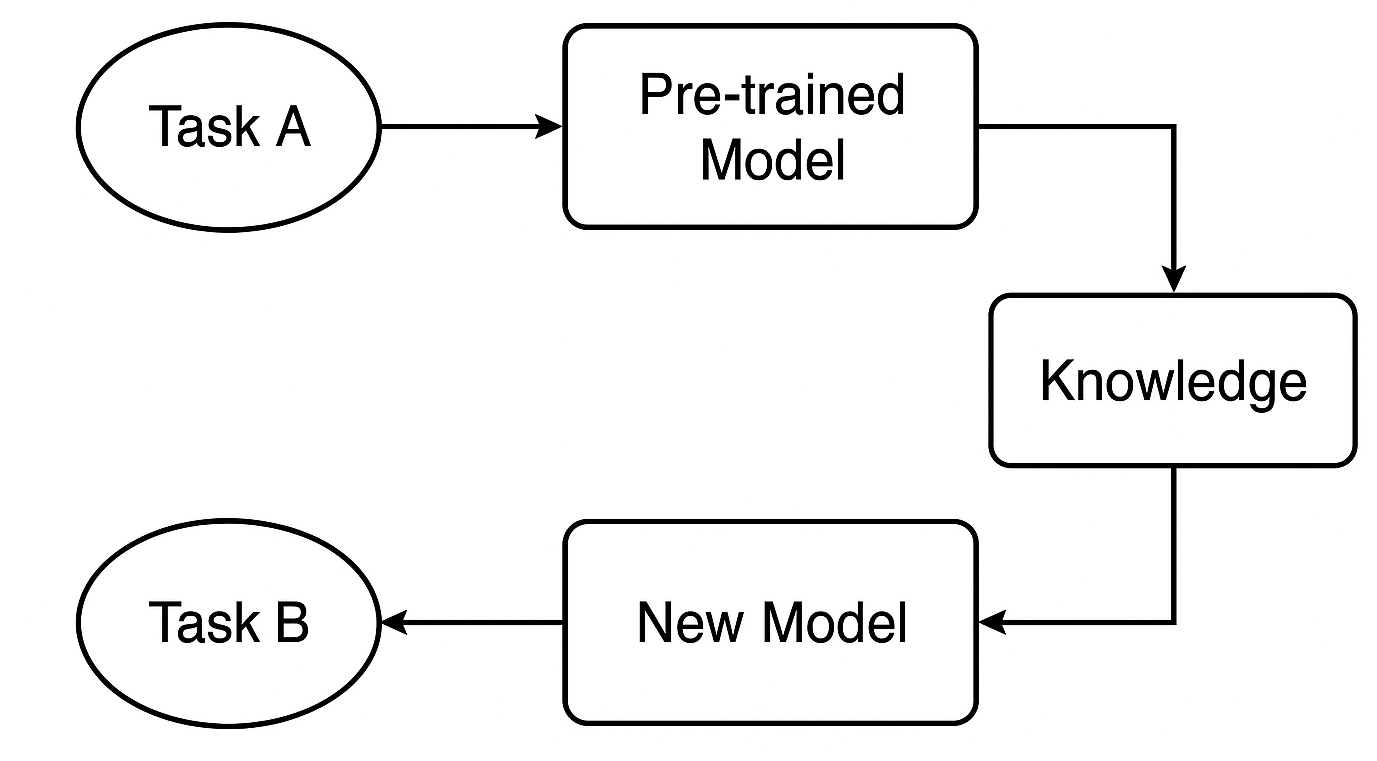
What is a pre-trained model?
We start with a model that’s already been trained on a large dataset for Task A. This model has learned to recognize general patterns and features that are useful for similar tasks.
In trading, for example, it could be a model trained on one strategy or symbol, which already understands common market behaviors that also appear in other forex instruments.
How is knowledge transferred?
If we’re using a neural network like a CNN or RNN, we can take the early layers — the ones that capture general features — and reuse them. These layers act like a foundation, detecting broad patterns that are helpful in both the original and new tasks.
Fine-tuning for the new task
Next, we adjust the model for Task B — maybe another instrument or strategy — by tuning certain layers or parameters so it performs well with the new data. This step customizes the model to the new situation.
Why Use Transfer Learning?
1. Faster training
Instead of starting from scratch, we reuse learned features. This significantly reduces training time — especially in deep learning, where saving hours or even days of computation can make a huge difference.
2. Often improves accuracy
Models that use transfer learning tend to perform better, especially when labeled data is limited. The pre-trained model already knows how to detect important signals like trading setups or indicators, which helps it make smarter decisions in the new task.
3. Works even with small or noisy datasets
Let’s face it: getting good historical or tick data in MetaTrader 5 for some symbols is tough. Some instruments simply don’t have enough data. But by using a model trained on a richer dataset, we can avoid overfitting and still build a strong model, even with limited data.
4. Reusable knowledge across instruments
Markets often behave similarly on a technical level. So instead of training a new model for every symbol, we can share and reuse knowledge across instruments — saving time and improving consistency.
A Simple Base Model
Let's train a simple Random forest classifier to get a starting point (a base model). We can use the OHLC (Open, High, Low, and Close) values for simplicity.
We start by collecting OHLC values across various major and minor forex instruments, adding some metals in the mix too.
#include <pandas.mqh> //https://www.mql5.com/en/articles/17030

input datetime start_date = D'2005.01.01';
input datetime end_date = D'2023.01.01';

input string symbols = "EURUSD|GBPUSD|AUDUSD|USDCAD|USDJPY|USDCHF|NZDUSD|EURNZD|AUDNZD|GBPNZD|NZDCHF|NZDJPY|NZDCAD|XAUUSD|XAUJPY|XAUEUR|XAUGBP";
input ENUM_TIMEFRAMES timeframe = PERIOD_D1;
//+------------------------------------------------------------------+
//| Script program start function                                    |
//+------------------------------------------------------------------+
void OnStart()
  {

   string SymbolsArr[];
   ushort sep = StringGetCharacter("|",0);
   if (StringSplit(symbols, sep, SymbolsArr)<0)
     {
       printf("%s failed to split the symbols, Error %d",__FUNCTION__,GetLastError());
       return;
     }

//---

   vector open, high, low, close;
   for (uint i=0; i<SymbolsArr.Size(); i++)
    {
      string symbol = SymbolsArr[i];
      if (!SymbolSelect(symbol, true))
         {
            printf("%s failed to select symbol %s, Error = %d",__FUNCTION__,symbol,GetLastError());
            continue;
         }

    //---

      open.CopyRates(symbol, timeframe, COPY_RATES_OPEN, start_date, end_date);
      high.CopyRates(symbol, timeframe, COPY_RATES_HIGH, start_date, end_date);
      low.CopyRates(symbol, timeframe, COPY_RATES_LOW, start_date, end_date);
      close.CopyRates(symbol, timeframe, COPY_RATES_CLOSE, start_date, end_date);

      CDataFrame df;

      df.insert("Open", open);
      df.insert("High", high);
      df.insert("Low", low);
      df.insert("Close", close);

      df.to_csv(StringFormat("Fxdata.%s.%s.csv",symbol,EnumToString(timeframe)), true);
    }
  }
After collecting the data, we can access the CSV files inside a Python script right away.
def getXandY(symbol: str, timeframe: str, lookahead: int) -> tuple:

    df = pd.read_csv(f"/kaggle/input/ohlc-eurusd/Fxdata.{symbol}.{timeframe}.csv")

    # Target variable

    df["future_close"] = df["Close"].shift(-lookahead)
    df.dropna(inplace=True)

    df["Signal"] = (df["future_close"] > df["Close"]).astype(int)

    # Splitting data into X and y

    X = df.drop(columns=[
        "future_close",
        "Signal"
    ])

    y = df["Signal"]

    return (X, y)
After reading the CSV file the function getXandY prepares the target variable based on a simple logic, if the next bar close is greater than the current close price that is a bullish signal, and the opposite when the next bar close is below the current close.
Let us make a function for training a model based on X and y data and return a trained model in a Scikit-learn pipeline.
def trainSymbol(X_train: pd.DataFrame, y_train: pd.DataFrame) -> Pipeline:

    # Training a model

    classifier = RandomForestClassifier(n_estimators=100, min_samples_split=3, max_depth = 5)

    pipeline = Pipeline([
        ("scaler", RobustScaler()),
        ("classifier", classifier)
    ])

    pipeline.fit(X_train, y_train)

    return pipeline
A function for evaluating this model across different instruments would be useful.
def evalSymbol(model: Pipeline, X: pd.DataFrame , y: pd.Series) -> int:

    # evaluating the model

    preds = model.predict(X)
    acc = accuracy_score(y, preds)

    return acc
Let's train our base model on EURUSD and then evaluate its performance on the rest of the symbols we have collected.
symbols = ["EURUSD","GBPUSD","AUDUSD","USDCAD","USDJPY","USDCHF","NZDUSD","EURNZD","AUDNZD","GBPNZD","NZDCHF","NZDJPY","NZDCAD","XAUUSD","XAUJPY","XAUEUR","XAUGBP"]

# training on EURUSD

lookahead = 1

X, y = getXandY(symbol=symbols[0], timeframe="PERIOD_H4", lookahead=lookahead)

X_train, X_test, y_train, y_test = train_test_split(X, y, random_state=42, shuffle=True)

model = trainSymbol(X_train, y_train)

# Evaluating on the rest of symbols

trained_symbol = symbols[0]

print(f"Trained on {trained_symbol}")
for symbol in symbols:
    X, y = getXandY(symbol=symbol, timeframe="PERIOD_H4", lookahead=1)

    acc = evalSymbol(model, X, y)
    print(f"--> {symbol} | acc: {acc}")
Outputs.
Trained on EURUSD
--> EURUSD | acc: 0.5478518727715607
--> GBPUSD | acc: 0.5009182736455464
--> AUDUSD | acc: 0.5026133634694165
--> USDCAD | acc: 0.4973701860284514
--> USDJPY | acc: 0.49477401129943505
--> USDCHF | acc: 0.5078731817539895
--> NZDUSD | acc: 0.4976826463824518
--> EURNZD | acc: 0.5071507150715071
--> AUDNZD | acc: 0.5005597760895641
--> GBPNZD | acc: 0.503459397596629
--> NZDCHF | acc: 0.4990389436737423
--> NZDJPY | acc: 0.4908841561794127
--> NZDCAD | acc: 0.5023507681974645
--> XAUUSD | acc: 0.48674396277970605
--> XAUJPY | acc: 0.4816082121471343
--> XAUEUR | acc: 0.4925268155442237
--> XAUGBP | acc: 0.49455864570737607
The model was 0.54 accurate on the symbol it was trained on, and the accuracy on the rest lay between 0.48 - 0.50, you might think this result doesn't deviate much from the one achieved on the training symbol so, this means the model operates well on symbols it wasn't trained on to say the least however, this is a terrible outcome.
Simply because a winning rate of 0.5 out of 1 (50% out of 100%) is like flipping a coin, your winning probability is 0.5 out of 1.
Despite the base model seeming like it's making some predictions on other instruments it wasn't trained on, we have a huge problem caused by continuous features (variables). Those OHLC values.
The Problem with Continuous Variables
Since we want to make our base model robust and universal, making it able to detect patterns and operate across various symbols, continuous variables features such as Open, High, Low, and Close price values are incompetent in this task because they offer no patterns other than a display of how the prices moved in the past.
Not to mention that each instrument has its price in a very different magnitude from the others. For example, today's closing prices look as follows:
| SYMBOL | DAILY CLOSING PRICE |
|---|---|
| USDJPY | 142.17 |
| EURUSD | 1.13839 |
| XAUUSD | 3305.02 |
This means that a model trained on each instrument might not be able to cope with others due to their differences in pricing.
Apart from not containing learnable patterns, models trained on continuous variables do require re-training frequently because markets reach new heights every day so we are going to have to train our models on a regular to keep up with the pace and update our models with new/recent information, this increases the computational cost which something that transfer learning aims to solve.
Only stationary variables are the ones capable of assisting machine learning models in capturing and becoming relevant across different markets, simply because their mean, variance, and autocorrelation do not change over time (they remain constant). This can be observed across different instruments.
If we want to leverage transfer learning, then all features such as indicators and patterns extracted from the market in our independent variables must either be constant or stationary.
For example, if you take indicators reading from the RSI indicator on any instrument the values will still be between 0 - 100, this is crucial for capturing patterns.
Feature engineering
There are plenty of techniques we can deploy to get stationary variables but for now, we can use a few techniques to craft our data such as calculating the percentage change on the closing price, differencing each OHLC value, and using some stationary indicators.
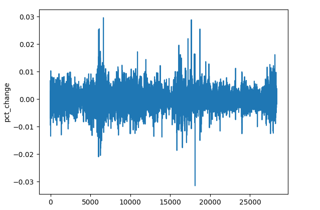
(a): Percentage change on Closing price
res_df["pct_change"] = df["Close"].pct_change()
Despite the difference in magnitude of the price across different symbols (instruments), the percentage change values will always be constant, making them a good universal feature for pattern detection.
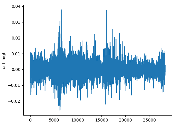
(b): Differencing each OHLC value
res_df["diff_open"] = df["Open"].diff()
res_df["diff_high"] = df["High"].diff()
res_df["diff_low"] = df["Low"].diff()
res_df["diff_close"] = df["Close"].diff()
The diff() method calculates the difference between the current element and the previous 1 (by default). This feature can help us detect how price changes on each bar compared to the previous one on every instrument.
(c): Stationary Indicators
We can add some momentum and oscillator indicators that exhibit stationary outcomes.
Indicator | Range of Values |
|---|---|
# Relative Strength Index (RSI) res_df['rsi'] = ta.momentum.RSIIndicator(df["Close"], window=14).rsi() | From 0 to 100. |
# Stochastic Oscillator (Stoch) res_df['stoch_k'] = ta.momentum.StochasticOscillator(df['High'], df['Low'], df['Close'], window=14).stoch() | From 0 to 100. |
# Moving Average Convergence Divergence (MACD) res_df['macd'] = ta.trend.MACD(df["Close"]).macd() | Small positive and negative values, Usually from -0.1 to +0.1. |
# Commodity Channel Index (CCI) res_df['cci'] = ta.trend.CCIIndicator(df['High'], df['Low'], df['Close'], window=20).cci() | Typically from -300 to +300. |
# Rate of Change (ROC) res_df['roc'] = ta.momentum.ROCIndicator(df["Close"], window=12).roc() | Unbounded, can either be negative or positive. |
# Ultimate Oscillator (UO) res_df['uo'] = ta.momentum.UltimateOscillator(df['High'], df['Low'], df['Close'], window1=7, window2=14, window3=28).ultimate_oscillator() | From 0 to 100. |
# Williams %R res_df['williams_r'] = ta.momentum.WilliamsRIndicator(df['High'], df['Low'], df['Close']).williams_r() | From -100 to 0. |
# Average True Range (ATR) res_df['atr'] = ta.volatility.AverageTrueRange(df['High'], df['Low'], df['Close'], window=14).average_true_range() | Unbounded small positive values. |
# Awesome Oscillator (AO) res_df['ao'] = ta.momentum.AwesomeOscillatorIndicator(df['High'], df['Low']).awesome_oscillator() | Unbounded small values, typically from -0.1 to +0.1 |
# Average Directional Index (ADX) res_df['adx'] = ta.trend.ADXIndicator(df['High'], df['Low'], df['Close'], window=14).adx() | From 0 to 100. |
# True Strength Index (TSI) res_df['tsi'] = ta.momentum.TSIIndicator(df['Close'], window_slow=25, window_fast=13).tsi() | Typically from -100 to +100. |
These are just a few stationary variables, feel free to add more of your choice.
All these methods and operations can be wrapped in a standalone function.
def getStationaryVars(df: pd.DataFrame) -> pd.DataFrame:

    res_df = pd.DataFrame()

    res_df["pct_change"] = df["Close"].pct_change()
    res_df["diff_open"] = df["Open"].diff()
    res_df["diff_high"] = df["High"].diff()
    res_df["diff_low"] = df["Low"].diff()
    res_df["diff_close"] = df["Close"].diff()

    # Relative Strength Index (RSI)
    res_df['rsi'] = ta.momentum.RSIIndicator(df["Close"], window=14).rsi()

    # Stochastic Oscillator (Stoch)
    res_df['stoch_k'] = ta.momentum.StochasticOscillator(df['High'], df['Low'], df['Close'], window=14).stoch()

    # Moving Average Convergence Divergence (MACD)
    res_df['macd'] = ta.trend.MACD(df["Close"]).macd()

    # Commodity Channel Index (CCI)
    res_df['cci'] = ta.trend.CCIIndicator(df['High'], df['Low'], df['Close'], window=20).cci()

# .... See the code in the notebook in the attachments and above
# ....
# ....

    # True Strength Index (TSI)
    res_df['tsi'] = ta.momentum.TSIIndicator(df['Close'], window_slow=25, window_fast=13).tsi()

    return res_df
Now let's create a base model that will be used to transfer knowledge from one instrument to another.
Transfer Learning
Transfer learning is usually done on deep models, Convolutional Neural Networks (CNNs) mostly. Simply because CNNs excel at pattern detection, this capability allows them to identify similar patterns which can then be transferred to different aspects within the same domain.
Let's wrap a Convolutional Neural Network (CNN) model within a function named trainCNN.
import tensorflow as tf
from tensorflow.keras import layers, models, Model
from tensorflow.keras.callbacks import EarlyStopping
def trainCNN(train_set: tuple, val_set: tuple, learning_rate: float=1e-3, epochs: int=100, batch_size: int=32):

    X_train, y_train = train_set
    X_val, y_val = val_set

    input_shape = X_train.shape[1:]
    num_classes = len(np.unique(y_train))

    model = models.Sequential([
        layers.Input(shape=input_shape),

        layers.Conv1D(64, kernel_size=3, activation='relu', padding='same'),
        layers.Conv1D(64, kernel_size=3, activation='relu', padding='same'),
        layers.GlobalAveragePooling1D(),

        layers.Dense(32, activation='tanh'),
        layers.Dense(num_classes, activation='softmax')
    ])

    # Compile with Adam optimizer
    model.compile(
        optimizer=tf.keras.optimizers.Adam(learning_rate=learning_rate),
        loss='categorical_crossentropy',
        metrics=['accuracy']
    )

    # Early stopping callback
    early_stop = EarlyStopping(
        monitor='val_loss',    # Watch validation loss
        patience=10,            # Stop if no improvement
        restore_best_weights=True
    )

    # Train the model
    model.fit(
        X_train, y_train,
        validation_data=(X_val, y_val),
        epochs=epochs,
        batch_size=batch_size,
        callbacks=[early_stop],
        verbose=1
    )

    # Save trained weights
    model.save_weights('cnn_pretrained.weights.h5')

    return model
This sequential model has two Convolutional 1D layers that can help us in extracting the features from the input sequence.
The global average pooling layer is introduced to reduce the sequences so that they can be fed to a dense layer (FNN layer) with a tanh activation function.
The last layer has a softmax activation function for returning predicted probabilities for each class.
We save the models' weight as they are they represent all learned patterns from the data, these weights can be passed to a preceding model.
Using EURUSD from a 4-hour timeframe, we can collect OHLC values from the original data frame.
lookahead = 1
trained_symbol = symbols[0]
timeframe = "PERIOD_H4"

df = pd.read_csv(f"/kaggle/input/ohlc-eurusd/Fxdata.{trained_symbol}.{timeframe}.csv")

stationary_df = getStationaryVars(df)

stationary_df["Close"] = df["Close"] # add the close price for crafting the target variable

X, y = getXandY(df=stationary_df, lookahead=lookahead)
Again, function getXandY creates a target variable using the Close values and based on the lookahead value given (1 in this case).
def getXandY(df: pd.DataFrame, lookahead: int) -> tuple:

    # Target variable

    df["future_close"] = df["Close"].shift(-lookahead)
    df.dropna(inplace=True)

    df["Signal"] = (df["future_close"] > df["Close"]).astype(int) # if next bar closed above the current one, thats a bullish signal otherwise bearish

    # Splitting data into X and y

    X = df.drop(columns=[
        "Close",
        "future_close",
        "Signal"
    ])

    y = df["Signal"]

    return (X, y)
We have to split the data into training and validation (testing) sets, then standardize the outcome using a scaler of choice, in this case, the Robust Scaler.
X_train, X_test, y_train, y_test = train_test_split(X, y, test_size=0.3, shuffle=False, random_state=42)

# Scalling the data

scaler = RobustScaler()

X_train_scaled = scaler.fit_transform(X_train)
X_test_scaled = scaler.transform(X_test)
Since Convolutional Neural Networks (CNNs) require a 3D input/data, we can process this data to be within a specific window for temporal pattern detection over this specific horizon.
def create_sequences(X, Y, time_step):

    if len(X) != len(Y):
        raise ValueError("X and y must have the same length")

    X = np.array(X)
    Y = np.array(Y)

    Xs, Ys = [], []

    for i in range(X.shape[0] - time_step):
        Xs.append(X[i:(i + time_step), :])  # Include all features with slicing
        Ys.append(Y[i + time_step])

    return np.array(Xs), np.array(Ys)
# Prepare data within a window

window = 10

X_train_seq, y_train_seq = create_sequences(X_train_scaled, y_train, window)
X_test_seq, y_test_seq = create_sequences(X_test_scaled, y_test, window)
One-hot encoding is crucial for the target variable in any classification problem involving neural networks as it helps them distinguish the classes.
# One-hot encode the labels for multi-class classification

y_train_encoded = to_categorical(y_train_seq, num_classes=num_classes)
y_test_encoded = to_categorical(y_test_seq, num_classes=num_classes)
Finally, we can train a base model.
base_model = trainCNN(train_set=(X_train_seq, y_train_encoded),
                 val_set=(X_test_seq, y_test_encoded),
                 learning_rate = 0.01,
                 epochs = 1000,
                 batch_size =32)

print("Test acc: ", base_model.evaluate(X_test_seq, y_test_encoded)[1])
Outputs.
Epoch 1/1000
620/620 ━━━━━━━━━━━━━━━━━━━━ 4s 4ms/step - accuracy: 0.4994 - loss: 0.6990 - val_accuracy: 0.5023 - val_loss: 0.6938
Epoch 2/1000
620/620 ━━━━━━━━━━━━━━━━━━━━ 1s 2ms/step - accuracy: 0.4976 - loss: 0.6939 - val_accuracy: 0.5023 - val_loss: 0.6936
Epoch 3/1000
620/620 ━━━━━━━━━━━━━━━━━━━━ 1s 2ms/step - accuracy: 0.4977 - loss: 0.6940 - val_accuracy: 0.5023 - val_loss: 0.6938
Epoch 4/1000
620/620 ━━━━━━━━━━━━━━━━━━━━ 1s 2ms/step - accuracy: 0.5034 - loss: 0.6937 - val_accuracy: 0.4977 - val_loss: 0.6962
...
...
Epoch 16/1000
620/620 ━━━━━━━━━━━━━━━━━━━━ 1s 2ms/step - accuracy: 0.5039 - loss: 0.6934 - val_accuracy: 0.5023 - val_loss: 0.6932
Epoch 17/1000
620/620 ━━━━━━━━━━━━━━━━━━━━ 1s 2ms/step - accuracy: 0.4988 - loss: 0.6940 - val_accuracy: 0.4977 - val_loss: 0.6937
Epoch 18/1000
620/620 ━━━━━━━━━━━━━━━━━━━━ 1s 2ms/step - accuracy: 0.5013 - loss: 0.6943 - val_accuracy: 0.5023 - val_loss: 0.6931
266/266 ━━━━━━━━━━━━━━━━━━━━ 0s 1ms/step - accuracy: 0.5037 - loss: 0.6931
Test acc:  0.5022971034049988
Great, we just trained a base model on EURUSD and achieved a 0.502 overall accuracy.
Now, let's use this model to transfer and share knowledge on other models trained on different instruments and see how that goes.
for symbol in symbols:

    if symbol == trained_symbol: # skip transfer learning on the trained symbol
        continue

    print(f"Symbol: {symbol}")

    df = pd.read_csv(f"/kaggle/input/ohlc-eurusd/Fxdata.{symbol}.{timeframe}.csv")

    stationary_df = getStationaryVars(df)
    stationary_df["Close"] = df["Close"] # we add the close price for crafting the target variable

    X, y = getXandY(df=stationary_df, lookahead=lookahead)

    X_train, X_test, y_train, y_test = train_test_split(X, y, test_size=0.3, shuffle=False, random_state=42)

    # Scalling the data

    scaler = RobustScaler()

    X_train_scaled = scaler.fit_transform(X_train)
    X_test_scaled = scaler.transform(X_test)

    # Prepare data within a window

    window = 10

    X_train_seq, y_train_seq = create_sequences(X_train_scaled, y_train, window)
    X_test_seq, y_test_seq = create_sequences(X_test_scaled, y_test, window)

    # One-hot encode the labels for multi-class classification

    y_train_encoded = to_categorical(y_train_seq, num_classes=num_classes)
    y_test_encoded = to_categorical(y_test_seq, num_classes=num_classes)

    # Freeze all layers except the last one
    for layer in base_model.layers[:-1]:
        layer.trainable = False

    # Create new model using the base model's architecture
    model = models.clone_model(base_model)
    model.set_weights(base_model.get_weights())

    # Recompile with lower learning rate
    model.compile(optimizer=tf.keras.optimizers.Adam(0.01),
                  loss='categorical_crossentropy',
                  metrics=['accuracy'])

    early_stop = EarlyStopping(monitor='val_loss', patience=10, restore_best_weights=True)

    history = model.fit(X_train_seq, y_train_encoded,
                       validation_data=(X_test_seq, y_test_encoded),
                       epochs=1000,  # More epochs for fine-tuning
                       batch_size=32,
                       callbacks=[early_stop],
                       verbose=1)

    print("Test acc:", model.evaluate(X_test_seq, y_test_encoded)[1])
The same processes are repeated for splitting the data, creating sequential data, and encoding the target variable. The operations are only specified for each symbol.
To transfer the knowledge from the base model we build another model based on the base one, the crucial thing here is to freeze some of the CNN layers.
We freeze all the layers of a CNN model except the last one because we want our model to preserve the patterns learned from the base data. By freezing some of the layers we prevent useful features from being destroyed when retraining this model on new data.
We leave the final layer unfrozen because we want the final layer's weights to recalibrate to new decision boundaries for each symbol, so basically, we provide the model with new distributions on the target variable and let it determine the relationships between the learned patterns from the base model and what's on the target variable on this new data.
We also clone the model architecture from the base model to the current model and assign its weights to the new model. Remember we saved the weights in the function trainCNN, you can load the weights from a file when you import the model from somewhere or load the model's weights directly from the model object if the base model is in the same Python script or file just like above.
In the end, we compile the model on market data from a different instrument other than the one used when training the base model, other parameters can be modified as well.
Below is the accuracy achieved across different forex symbols.
| SYMBOL | GBPUSD | AUDUSD | USDCAD | USDJPY | USDCHF | NZDUSD | EURNZD | AUDNZD | GBPNZD | NZDCHF | NZDJPY | NZDCAD | XAUUSD | XAUJPY | XAUEUR | XAUGBP |
| ACCURACY | 0.505 | 0.506 | 0.501 | 0.516 | 0.506 | 0.497 | 0.505 | 0.502 | 0.504 | 0.505 | 0.51 | 0.505 | 0.506 | 0.514 | 0.507 | 0.504 |
Now this outcome doesn't tell us much, let us incorporate the classification report to analyze this outcome in detail.
preds = base_model.predict(X_test_seq)
pred_indices = preds.argmax(axis=1)
pred_class_labels = [classes_in_y[i] for i in pred_indices]

print("Classification report\n", classification_report(pred_class_labels, y_test_seq))
The classification report on the base model.
Classification report
               precision    recall  f1-score   support

           0       1.00      0.50      0.66      8477
           1       0.00      0.00      0.00         0

    accuracy                           0.50      8477
   macro avg       0.50      0.25      0.33      8477
weighted avg       1.00      0.50      0.66      8477
This outcome indicates a terrible outcome. A heavily biased classification report was produced by the model.
This indicates that we have bias in our model which could be caused by our model or data.
There are a couple of ways to address this bias situation as we discussed in this prior article, but, for now, let's do a couple of things:
(a): Let's add class weights to fix class imbalance if it exists in our data.
from sklearn.utils.class_weight import compute_class_weight
def trainCNN:

#....
#....

    y_train_integers = np.argmax(y_train, axis=1) # return to non-one hot encoded
    class_weights = compute_class_weight('balanced',
                                       classes=np.unique(y_train_integers),
                                       y=y_train_integers)
    class_weight_dict = {i: weight for i, weight in enumerate(class_weights)}


    # Train the model
    model.fit(
        X_train, y_train,
        validation_data=(X_val, y_val),
        epochs=epochs,
        batch_size=batch_size,
        callbacks=[early_stop],
        class_weight=class_weight_dict,
        verbose=1
    )
(b): Let's add another convolutional layer and increase the number of neurons in the dense layer to help in capturing complicated patterns.
def trainCNN:

# ...
# ...

    model = models.Sequential([
        layers.Input(shape=input_shape),

        layers.Conv1D(64, kernel_size=3, activation='relu', padding='same'),
        layers.Conv1D(64, kernel_size=3, activation='relu', padding='same'),
        layers.Conv1D(32, kernel_size=3, activation='relu', padding='same'),
        layers.GlobalAveragePooling1D(),

        layers.Dense(128, activation='relu'),
        layers.Dense(num_classes, activation='softmax')
    ])
(c): Since this is a binary classification problem, we have two classes only in our target variable. 0 for sell signals and 1 for buy signals, let's change the loss function to 'binary_crossentropy' and the evaluation metric to 'binary_accuracy'.
    # Compile with Adam optimizer
    model.compile(
        optimizer=tf.keras.optimizers.Adam(learning_rate=learning_rate),
        loss='binary_crossentropy',
        metrics=['binary_accuracy']
    )
When a CNN model was re-trained, the values looked a lot better.
....
....
310/310 ━━━━━━━━━━━━━━━━━━━━ 1s 3ms/step - binary_accuracy: 0.5257 - loss: 0.6920 - val_binary_accuracy: 0.5043 - val_loss: 0.6933
Epoch 7/100
310/310 ━━━━━━━━━━━━━━━━━━━━ 1s 3ms/step - binary_accuracy: 0.5259 - loss: 0.6918 - val_binary_accuracy: 0.5027 - val_loss: 0.6934
Epoch 8/100
310/310 ━━━━━━━━━━━━━━━━━━━━ 1s 2ms/step - binary_accuracy: 0.5283 - loss: 0.6915 - val_binary_accuracy: 0.5042 - val_loss: 0.6936
Epoch 9/100
310/310 ━━━━━━━━━━━━━━━━━━━━ 1s 2ms/step - binary_accuracy: 0.5284 - loss: 0.6912 - val_binary_accuracy: 0.5028 - val_loss: 0.6937
Epoch 10/100
310/310 ━━━━━━━━━━━━━━━━━━━━ 1s 2ms/step - binary_accuracy: 0.5315 - loss: 0.6909 - val_binary_accuracy: 0.5036 - val_loss: 0.6938
Epoch 11/100
310/310 ━━━━━━━━━━━━━━━━━━━━ 1s 2ms/step - binary_accuracy: 0.5295 - loss: 0.6907 - val_binary_accuracy: 0.5042 - val_loss: 0.6940
Epoch 12/100
310/310 ━━━━━━━━━━━━━━━━━━━━ 1s 3ms/step - binary_accuracy: 0.5298 - loss: 0.6904 - val_binary_accuracy: 0.5074 - val_loss: 0.6941
619/619 ━━━━━━━━━━━━━━━━━━━━ 1s 2ms/step - binary_accuracy: 0.5101 - loss: 0.6926
265/265 ━━━━━━━━━━━━━━━━━━━━ 0s 1ms/step - binary_accuracy: 0.5018 - loss: 0.6933
Train acc: 0.5114434361457825 Test acc: 0.5050135850906372
265/265 ━━━━━━━━━━━━━━━━━━━━ 1s 2ms/step
Classification report
               precision    recall  f1-score   support

           0       0.58      0.50      0.54      4870
           1       0.43      0.51      0.47      3607

    accuracy                           0.51      8477
   macro avg       0.51      0.51      0.50      8477
weighted avg       0.52      0.51      0.51      8477
There was no specific reason for the modified parameters. I wanted to prove that just like any other neural network-based model, optimization and parameter tuning are very crucial.
The current outcome may not be the optimal solution as well because there is a lot we can discuss about CNNs and neural networks in general.
Let's proceed with the current parameters for now but feel free to tune these values to get a model that suits your needs.
Now that we have a base model that isn't so biased, we can use it to transfer its knowledge to other instruments and save all these models to ONNX format for the sake of observing the outcome provided by transfer learning in an actual trading environment.
Transfer Learning on a Trading Robot (EA)
To test transfer learning on a trading environment in MetaTrader 5, we have to save the models first in ONNX format and then load them using the MQL5 programming language.
Imports.
import onnxmltools
import tf2onnx
from skl2onnx import convert_sklearn
from skl2onnx.common.data_types import FloatTensorType
Functions
def saveCNN(model, window: int, features: int, filename: str):

    model.output_names = ["output"]
    # Specifying the input signature for the model
    spec = (tf.TensorSpec((None, window, features), tf.float16, name="input"),)

    # Convert the Keras model to ONNX format
    onnx_model, _ = tf2onnx.convert.from_keras(model, input_signature=spec, opset=14)

    # Save the ONNX model to a file
    with open(filename, "wb") as f:
        f.write(onnx_model.SerializeToString())
Since Keras models don't have a supported pipeline like the one we often use to wrap all preprocessing techniques alongside the Scikit-learn model, which makes it easier to save the model and all its steps in a single ONNX file, we have to save a Keras model and a scaler used separately as independent ONNX files.
def saveScaler(scaler, features: int, filename: str):

    # Convert to ONNX format
    initial_type = [("input", FloatTensorType([None, features]))]
    onnx_model = convert_sklearn(scaler, initial_types=initial_type, target_opset=14)


    with open(filename, "wb") as f:
        f.write(onnx_model.SerializeToString())
Now, we can call these functions when saving the base model and the preceding ones.
Saving the base model.
# ....
# ....

base_model = trainCNN(train_set=(X_train_seq, y_train_encoded),
                 val_set=(X_test_seq, y_test_encoded),
                 learning_rate = 0.01,
                 epochs = 1000,
                 batch_size =32)

saveCNN(model=base_model,
        window=window,
        features=X_train_seq.shape[2],
        filename=f"{trained_symbol}.basemodel.{timeframe}.onnx")

saveScaler(scaler=scaler,
           features=X_train.shape[1],
           filename=f"{trained_symbol}.{timeframe}.scaler.onnx")
Saving models trained under transfer learning.
for symbol in symbols:

# ...
# ...

    history = model.fit(X_train_seq, y_train_encoded,
                       validation_data=(X_test_seq, y_test_encoded),
                       epochs=1000,  # More epochs for fine-tuning
                       batch_size=32,
                       callbacks=[early_stop],
                       verbose=1)

    saveCNN(model=model,
        window=window,
        features=X_train_seq.shape[2],
        filename=f"basesymbol={trained_symbol}.symbol={symbol}.model.{timeframe}.onnx")


    saveScaler(scaler=scaler,
               features=X_train.shape[1],
               filename=f"{symbol}.{timeframe}.scaler.onnx")
After saving the files in the Common Folder, we can load them inside an Expert Advisor (EA) in a similar naming fashion.
#include <ta.mqh> //similar to ta in Python --> https://www.mql5.com/en/articles/16931
#include <pandas.mqh> //similar to Pandas in Python --> https://www.mql5.com/en/articles/17030
#include <CNN.mqh> //For loading Convolutional Neural networks in ONNX format --> https://www.mql5.com/en/articles/15259
#include <preprocessing.mqh> //For loading the scaler transformer
#include <Trade\Trade.mqh> //The trading module
#include <Trade\PositionInfo.mqh> //Position handling module

CCNNClassifier cnn;
RobustScaler scaler;
CTrade m_trade;
CPositionInfo m_position;

input string base_symbol = "EURUSD";
input string symbol_ = "USDJPY";
input ENUM_TIMEFRAMES timeframe = PERIOD_H4;
input uint window_ = 10;
input uint lookahead = 1;
input uint magic_number = 28042025;
input uint slippage = 100;

long classes_in_y_[] = {0, 1};
int OldNumBars = -1;
//+------------------------------------------------------------------+
//| Expert initialization function                                   |
//+------------------------------------------------------------------+
int OnInit()
  {
//---

  if (!MQLInfoInteger(MQL_TESTER))
   if (!ChartSetSymbolPeriod(0, symbol_, timeframe))
      {
         printf("%s Failed to set symbol_ = %s and timeframe = %s, Error = %d",__FUNCTION__,symbol_,EnumToString(timeframe), GetLastError());
         return INIT_FAILED;
      }

//---

   string filename = StringFormat("basesymbol=%s.symbol=%s.model.%s.onnx",base_symbol, symbol_, EnumToString(timeframe));
   if (!cnn.Init(filename, ONNX_COMMON_FOLDER))
      {
         printf("%s failed to load a CNN model in ONNX format from the common folder '%s', Error = %d",__FUNCTION__,filename,GetLastError());
         return INIT_FAILED;
      }

//---

   filename = StringFormat("%s.%s.scaler.onnx", symbol_, EnumToString(timeframe));
   if (!scaler.Init(filename, ONNX_COMMON_FOLDER))
      {
         printf("%s failed to load a scaler in ONNX format from the common folder '%s', Error = %d",__FUNCTION__,filename,GetLastError());
         return INIT_FAILED;
      }
 }
Since we have the equivalent of the TA - (Technical Analysis) module from Python in MQL5 which we discussed in this article. We can call the indicator functions and assign the outcome in a Python-Pandas-like data frame.
CDataFrame getStationaryVars(uint start = 1, uint bars = 50)
  {
    CDataFrame df; //Dataframe object

    vector open, high, low, close;
    open.CopyRates(Symbol(), Period(), COPY_RATES_OPEN, start, bars);
    high.CopyRates(Symbol(), Period(), COPY_RATES_HIGH, start, bars);
    low.CopyRates(Symbol(), Period(), COPY_RATES_LOW, start, bars);
    close.CopyRates(Symbol(), Period(), COPY_RATES_CLOSE, start, bars);

    vector pct_change = df.pct_change(close);
    vector diff_open = df.diff(open);
    vector diff_high = df.diff(high);
    vector diff_low = df.diff(low);
    vector diff_close = df.diff(close);

    df.insert("pct_change", pct_change);
    df.insert("diff_open", open);
    df.insert("diff_high", high);
    df.insert("diff_low", low);
    df.insert("diff_close", close);

    // Relative Strength Index (RSI)
    vector rsi = CMomentumIndicators::RSIIndicator(close);
    df.insert("rsi", rsi);

    // Stochastic Oscillator (Stoch)
    vector stock_k = CMomentumIndicators::StochasticOscillator(close,high,low).stoch;
    df.insert("stock_k", stock_k);

    // Moving Average Convergence Divergence (MACD)
    vector macd = COscillatorIndicators::MACDIndicator(close).main;
    df.insert("macd", macd);

    // Commodity Channel Index (CCI)
    vector cci = COscillatorIndicators::CCIIndicator(high,low,close);
    df.insert("cci", cci);

    // Rate of Change (ROC)
    vector roc = CMomentumIndicators::ROCIndicator(close);
    df.insert("roc", roc);

    // Ultimate Oscillator (UO)
    vector uo = CMomentumIndicators::UltimateOscillator(high,low,close);
    df.insert("uo", uo);

    // Williams %R
    vector williams_r = CMomentumIndicators::WilliamsR(high,low,close);
    df.insert("williams_r", williams_r);

    // Average True Range (ATR)
    vector atr = COscillatorIndicators::ATRIndicator(high,low,close);
    df.insert("atr", atr);

    // Awesome Oscillator (AO)
    vector ao = CMomentumIndicators::AwesomeOscillator(high,low);
    df.insert("ao", ao);

    // Average Directional Index (ADX)
    vector adx = COscillatorIndicators::ADXIndicator(high,low,close).adx;
    df.insert("adx", adx);

    // True Strength Index (TSI)
    vector tsi = CMomentumIndicators::TSIIndicator(close);
    df.insert("tsi", tsi);

    if (MQLInfoInteger(MQL_DEBUG))
      df.head();

    df = df.dropna(); //Drop not-a-number variables

    return df; //return the last rows = window from a dataframe which is the recent information fromthe market
 }
On every bar, we collect 50 bars back in time for indicator calculations starting at the recently closed bar at the index of 1.
The main reason for 50 bars is to give enough room for indicator calculations which are accompanied by NaN (Not a Number) values that we want to avoid.
The Awesome oscillator indicator is the one that looks in the past the most with a window2 value of 34, this means 50-34 = 16 is the number of eligible data that remains for our model.
Running this function in debug mode will provide you with an overview of the data in the Experts tab on MetaTrader 5.
MD      0       18:17:26.145    Transfer Learning EA (USDJPY,H4)        | Index | pct_change      | diff_open        | diff_high        | diff_low         | diff_close       | rsi     | stock_k     | macd     | cci     | roc     | uo      | williams_r     | atr     | ao      | adx            | tsi     |
FF      0       18:17:26.145    Transfer Learning EA (USDJPY,H4)        |     0 | nan             | 142.67000000     | 143.08800000     | 142.49100000     | 142.68300000     | nan     | nan         | nan      | nan     | nan     | nan     | nan            | nan     | nan     | 0.00000000     | nan     |
JO      0       18:17:26.146    Transfer Learning EA (USDJPY,H4)        |     1 | -0.25300842     | 142.68400000     | 142.84900000     | 142.28700000     | 142.32200000     | nan     | nan         | nan      | nan     | nan     | nan     | nan            | nan     | nan     | 0.00000000     | nan     |
IR      0       18:17:26.146    Transfer Learning EA (USDJPY,H4)        |     2 | 0.09977375      | 142.32300000     | 142.63500000     | 141.89900000     | 142.46400000     | nan     | nan         | nan      | nan     | nan     | nan     | nan            | nan     | nan     | 0.00000000     | nan     |
HF      0       18:17:26.146    Transfer Learning EA (USDJPY,H4)        |     3 | -0.00070193     | 142.46400000     | 142.71900000     | 142.34400000     | 142.46300000     | nan     | nan         | nan      | nan     | nan     | nan     | nan            | nan     | nan     | 0.00000000     | nan     |
GJ      0       18:17:26.146    Transfer Learning EA (USDJPY,H4)        |     4 | -0.04702976     | 142.37400000     | 142.47200000     | 142.18600000     | 142.39600000     | nan     | nan         | nan      | nan     | nan     | nan     | nan            | nan     | nan     | 0.00000000     | nan     |
IJ      0       18:17:26.146    Transfer Learning EA (USDJPY,H4)        |  ...  |
NR      0       18:17:26.146    Transfer Learning EA (USDJPY,H4)        |    45 | -0.22551954     | 142.33800000     | 142.38800000     | 141.98200000     | 142.01700000     | 28.79606321 | 1.70731707  | 0.20202343 | -149.46898289 | -0.42629273 | 28.03714657 | -48.58934169   | 0.58185714 | 0.84359706 | 29.65580624    | 8.31951160 |
NJ      0       18:17:26.146    Transfer Learning EA (USDJPY,H4)        |    46 | 0.16054416      | 141.97800000     | 142.31600000     | 141.96400000     | 142.24500000     | 35.49705652 | 13.58800774 | 0.12993025 | -131.96513868 | -0.57316604 | 34.81743660 | -43.09139137   | 0.56978571 | 0.51217941 | 28.18573720    | 4.78996901 |
HQ      0       18:17:26.146    Transfer Learning EA (USDJPY,H4)        |    47 | 0.19543745      | 142.24500000     | 142.58100000     | 142.12400000     | 142.52300000     | 43.03880625 | 27.03094778 | 0.09414295 | -86.63856716 | -0.76174826 | 43.61239023 | -36.38775018   | 0.57742857 | 0.21773529 | 26.19967843    | 3.09202782 |
FH      0       18:17:26.146    Transfer Learning EA (USDJPY,H4)        |    48 | 0.04771160      | 142.52300000     | 142.61500000     | 142.29800000     | 142.59100000     | 44.85843867 | 30.31914894 | 0.07045611 | -66.64608781 | -0.57732936 | 49.55462139 | -34.74801061   | 0.56007143 | -0.01222353 | 24.37916904    | 2.01861384 |
MQ      0       18:17:26.146    Transfer Learning EA (USDJPY,H4)        |    49 | -0.19776844     | 142.59100000     | 142.75800000     | 142.25100000     | 142.30900000     | 38.91058297 | 16.68278530 | 0.02859940 | -70.14493704 | -0.77257229 | 41.99481159 | -41.54810707   | 0.52700000 | -0.13378529 | 23.02215655    | 0.05188403 |
Inside the OnTick function, the first thing that we do is get these stationary variables followed by the slicing operation which aims to ensure that the data or the number of bars received is within the required window we used when training a CNN model.
void OnTick()
  {
//---

   if (!isNewBar())
      return;

   CDataFrame x_df = getStationaryVars();

//--- Check if the number of rows received after indicator calculation is >= window size

   if ((uint)x_df.shape()[0]<window_)
      {
         printf("%s Fatal, Data received is less than the desired window=%u. Check your indicators or increase the number of bars in the function getSationaryVars()",__FUNCTION__,window_);
         DebugBreak();
         return;
      }

   ulong rows = (ulong)x_df.shape()[0];
   ulong cols = (ulong)x_df.shape()[1];

   //printf("Before scaled shape = (%I64u, %I64u)",rows, cols);

   matrix x = x_df.iloc((rows-window_), rows-1, 0, cols-1).m_values;
 }
Now that we have a sliced matrix with 10 rows similar to the window value and 16 features we used during training, we can pass this data to the loaded RobustScaler before passing it to the CNN model for final predictions.
matrix x_scaled = scaler.transform(x); //Transform the data, very important

long signal = cnn.predict(x_scaled, classes_in_y_).cls; //Predicted class
Finally, using the signal obtained from the model, we can make a simple trading strategy that when the signal received from the model equals to 1 (bullish signal), we open a buy trade and do the opposite when a signal received equals to 0 (bearish signal), we open a sell trade.
Each trade will be closed after the number of bars similar to the lookahead value has passed in the current timeframe.
//--- Trading functionality

   MqlTick ticks;
   if (!SymbolInfoTick(Symbol(), ticks))
      {
         printf("Failed to obtain ticks information, Error = %d",GetLastError());
         return;
      }

   double volume_ = SymbolInfoDouble(Symbol(), SYMBOL_VOLUME_MIN);

   if (signal == 1) //Check if there are is atleast a special pattern before opening a trade
     {
        if (!PosExists(POSITION_TYPE_BUY) && !PosExists(POSITION_TYPE_SELL))
            m_trade.Buy(volume_, Symbol(), ticks.ask,0,0);
     }

   if (signal == 0) //Check if there are is atleast a special pattern before opening a trade
     {
        if (!PosExists(POSITION_TYPE_SELL) && !PosExists(POSITION_TYPE_BUY))
            m_trade.Sell(volume_, Symbol(), ticks.bid,0,0);
     }

    CloseTradeAfterTime((Timeframe2Minutes(Period())*lookahead)*60); //Close the trade after a certain lookahead and according the the trained timeframe
That's it, let's run this trading robot on several instruments that we used during this transfer learning process and observe their predictive outcome from January 1st, 2023 to January 1st, 2025.
Timeframe: PERIOD_H4. Modelling: 1 Minute OHLC.
Symbol: XAUEUR
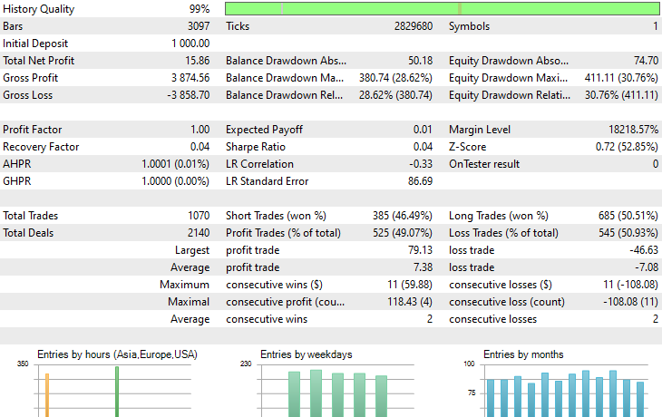
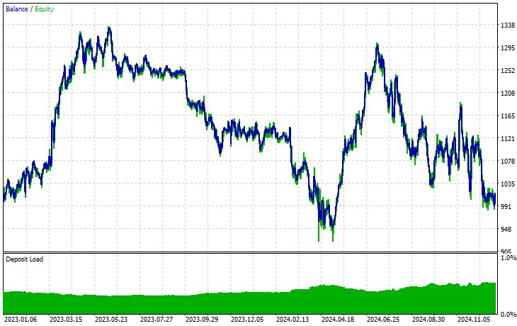
Symbol: XAUUSD
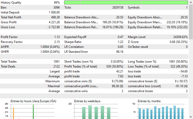
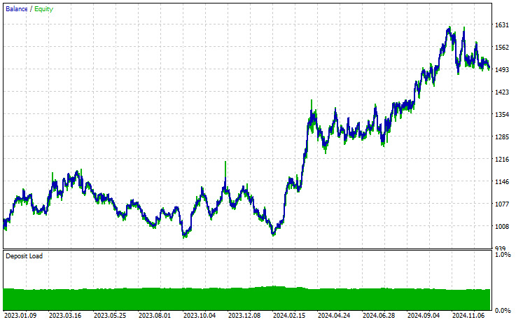
Out of 17 instruments we used during transfer learning on a base model trained on EURUSD, only 2 instruments had promising results. The rest were complete garbage.
This could mean two things, one is that patterns observed on EURUSD have a strong relationship or similarities to those displayed on XAUUSD and XAUEUR. It does make sense because these two instruments both have EUR and USD which makes up the base symbol EURUSD.
Secondly, this could also mean that we have suboptimal CNN models as we haven't optimized our models to find the best combination of the model's architecture and parameters, not to mention we haven't even exercised different base symbols and observed the outcomes on others.
We could have done a couple of things, but that's beyond the scope of this article. I leave that to you.
Final Thoughts
We are in the golden age of Artificial Intelligence and machine learning, this technology is advancing at a greater pace than anticipated all thanks to Open-source you can now build superb models on top of existing ones with a few lines of code, this is what we simply call transfer learning.
While we have these massive open-source models in computer vision and image-related tasks such as ResNet50, MobileNet, etc. Which has enabled developers to get on the edge and get meaningful AI solutions, the financial space is yet to be explored in the open-source aspect.
This article was aimed to open your eyes tp the possibility of transfer learning and how it might look like in this space as a starting point to help you build massive models to help us figure out financial markets by leveraging common patterns available across various instruments.
Good luck.
Attachments Table
Filename | Description/Usage |
|---|---|
| Expert\Transfer Learning EA.mq5 | The main Expert advisor for testing transfer learning models in a trading environment. |
| Include\CNN.mqh | A library for loading and deploying CNN models in in .onnx files In MQL5. |
Include\pandas.mqh | Python-Like Pandas library for data manipulation and storage |
Include\preprocessing.mqh | Contains classes for loading, scaling techniques data transformers present in .onnx format. |
Include\ta.mqh | A library with a plug-and-play approach for working with indicators in MQL5. |
Scripts\CollectData.mqh | A script for collecting and saving to CSV files OHLC data across various instruments. |
| Python\forex-transfer-learning.ipynb | A Python script (Jupyter Notebook) for executing all the python code described in this article. |
Common\Files\*scaler.onnx | Data preprocessing scalers saved in ONNX formatted files. |
Common\Files\*.onnx | CNN models saved in ONNX formatted files. |
Warning: All rights to these materials are reserved by MetaQuotes Ltd. Copying or reprinting of these materials in whole or in part is prohibited.
This article was written by a user of the site and reflects their personal views. MetaQuotes Ltd is not responsible for the accuracy of the information presented, nor for any consequences resulting from the use of the solutions, strategies or recommendations described.

- Free trading apps
- Over 8,000 signals for copying
- Economic news for exploring financial markets
You agree to website policy and terms of use