
Neural Networks Made Easy (Part 97): Training Models With MSFformer

Introduction
In the previous article we built the main modules of the MSFformer model, including CSCM and Skip-PAM. The CSCM module constructs a feature tree of the analyzed time series, while Skip-PAM extracts information from time series at multiple scales using attention mechanism based on a temporal feature tree. In this article, we will continue that work by training the model and evaluating its performance on real-world data using the MetaTrader 5 Strategy Tester.
1. Model architecture
Before proceeding with model training, we need to complete a number of preparatory steps. First and foremost, we must define the model architecture. The MSFformer method was designed for time series forecasting tasks. Accordingly, we will integrate it into the Environmental State Encoder model, alongside several other similar methods.
1.1 Architecture of the Environmental State Encoder
The architecture of the Environmental State Encoder is defined in the CreateEncoderDescriptions method. This method takes a pointer to a dynamic array object as a parameter, where we will specify the model architecture.
bool CreateEncoderDescriptions(CArrayObj *encoder)
  {
//---
   CLayerDescription *descr;
//---
   if(!encoder)
     {
      encoder = new CArrayObj();
      if(!encoder)
         return false;
     }
In the method body, we check the relevance of the received pointer and, if necessary, create a new instance of the dynamic array.
Next, we move on to defining the architecture of the model. The input to the Encoder consists of "raw" data describing the current state of the environment. As usual, we use a basic fully connected layer without an activation function as the input layer. In this case, the use of an activation function is unnecessary since the raw input data will be directly written into the result buffer of the specified layer.
//--- Encoder
   encoder.Clear();
//--- Input layer
   if(!(descr = new CLayerDescription()))
      return false;
   descr.type = defNeuronBaseOCL;
   int prev_count = descr.count = (HistoryBars * BarDescr);
   descr.activation = None;
   descr.optimization = ADAM;
   if(!encoder.Add(descr))
     {
      delete descr;
      return false;
     }
Please note that the size of the input layer must precisely match the dimensions of the environmental state description tensor. Moreover, the description of the environmental state must remain identical at all stages of model training and deployment. For easier synchronization of parameters across the training and production stages, we will define two constants: BarDescr (the number of elements describing a single candlestick) and HistoryBars (the depth of the analyzed historical data). The product of these constants will determine the size of the input layer.
As mentioned above, we intend to feed "raw" (unprocessed) data into the model. On the one hand, this approach simplifies synchronization between the data preprocessing blocks in the training and operation programs, which is a significant advantage.
On the other hand, using unprocessed data can often reduce the efficiency of model training. This is due to the significant statistical variability between the different elements of the input data. To mitigate this issue, we will perform an initial preprocessing of the input data directly inside the model. This task will be performed by a batch normalization layer. According to the algorithm of this layer, the output data will have a mean value close to zero and a unit variance.
//--- layer 1
   if(!(descr = new CLayerDescription()))
      return false;
   descr.type = defNeuronBatchNormOCL;
   descr.count = prev_count;
   descr.batch = 1e4;
   descr.activation = None;
   descr.optimization = ADAM;
   if(!encoder.Add(descr))
     {
      delete descr;
      return false;
     }
We feed the preprocessed input data of the normalized time series into the feature extraction module CSCM.
//--- layer 2
   if(!(descr = new CLayerDescription()))
      return false;
   descr.type = defNeuronCSCMOCL;
   descr.count = HistoryBars;
   descr.window = BarDescr;
Note that feature extraction will be performed within the framework of univariate time series. In this context, the sequence length corresponds to the depth of the analyzed historical data, while the number of univariate sequences equals the size of the vector describing a single candlestick. However, in previous articles, when constructing the environmental state description tensor, we typically organized the data into a matrix where rows represented the analyzed bars and columns corresponded to features. Therefore, we will specify in the parameters of the CSCM module that the data should undergo a preliminary transposition.
descr.step = int(true);
We will extract features in 3 levels with analysis window sizes of 6, 5 and 4 bars.
     {
      int temp[] = {6, 5, 4};
      if(!ArrayCopy(descr.windows, temp))
         return false;
     }
We do not use the activation function. We will optimize the model parameters using the Adam method.
   descr.step = int(true);
   descr.activation = None;
   descr.optimization = ADAM;
   if(!encoder.Add(descr))
     {
      delete descr;
      return false;
     }
Next, according to the algorithm of the MSFformer method, comes the Skip-PAM module. In our implementation, we will add 3 consecutive Skip-PAM layers with the same configuration.
//--- layer 3 - 5
   if(!(descr = new CLayerDescription()))
      return false;
   descr.type = defNeuronSPyrAttentionMLKV;
   descr.count = HistoryBars;
   descr.window = BarDescr;
Here we specify a similar size of the sequence being analyzed. However, in this case, we are already working with a multimodal sequence.
We set the size of the internal vector of Query, Key and Value entity descriptions equal to 32 elements. The number of attention heads for the Key-Value tensor will be 2 times less.
   descr.window_out = 32;
     {
      int temp[] = {8, 4};
      if(!ArrayCopy(descr.heads, temp))
         return false;
     }
   descr.layers = 3;
   descr.activation = None;
   descr.optimization = ADAM;
   for(int l = 0; l < 3; l++)
      if(!encoder.Add(descr))
        {
         delete descr;
         return false;
        }
The pyramid of attention of each Skip-PAM will contain 3 levels. Here we also use the Adam method to optimize the model parameters.
At the output of the Skip-PAM module, we get a tensor whose size corresponds to the input data. The content of the tensor is adjusted by dependencies between the elements of the analyzed sequence. Next, we need to construct predictive trajectories for the continuation of the multimodal input time series. We will construct separate forecast trajectories for each univariate series in the analyzed multimodal sequence. To do this, we first transpose the data tensor obtained from the Skip-PAM module.
//--- layer 6
   if(!(descr = new CLayerDescription()))
      return false;
   descr.type = defNeuronTransposeOCL;
   descr.count = HistoryBars;
   descr.window = BarDescr;
   if(!encoder.Add(descr))
     {
      delete descr;
      return false;
     }
After that, we will use 2 consecutive convolutional layers, which will perform the role of an MLP for individual univariate sequences.
//--- layer 7
   if(!(descr = new CLayerDescription()))
      return false;
   descr.type = defNeuronConvOCL;
   descr.count = BarDescr;
   descr.window = HistoryBars;
   descr.step = HistoryBars;
   descr.window_out = LatentCount;
   descr.activation = LReLU;
   descr.optimization = ADAM;
   if(!encoder.Add(descr))
     {
      delete descr;
      return false;
     }
//--- layer 8
   if(!(descr = new CLayerDescription()))
      return false;
   descr.type = defNeuronConvOCL;
   descr.count = BarDescr;
   descr.window = LatentCount;
   descr.step = LatentCount;
   descr.window_out = NForecast;
   descr.optimization = ADAM;
   descr.activation = TANH;
   if(!encoder.Add(descr))
     {
      delete descr;
      return false;
     }
Please note that to implement the similarity to MLP in the above convolutional layers, we specify equal sizes of the analyzed window and its step. In the first case, it is equal to the depth of the sequence being analyzed. In the second case, it is equal to the number of filters of the previous layer. Also, the number of convolution blocks is equal to the number of analyzed univariate sequences. To introduce nonlinearity between convolutional layers, we use the LReLU activation function.
For the second convolutional layer, we set the number of filters equal to the size of the predicted sequence. In our case, it is specified by the NForecast constant.
Additionally, for the second convolutional layer, we use the hyperbolic tangent (TANH). This choice is deliberate. At the input stage of the model, we used a batch normalization layer to preprocess the data, ensuring unit variance and a mean value close to zero. According to the "three-sigma rule", approximately 2/3 of values for a normally distributed random variable lie within one standard deviation of the mean. Consequently, using TANH, which has a value range of (-1, 1), allows us to cover 68% of the analyzed variable's values while filtering outliers that fall beyond one standard deviation from the mean.
It is important to note that our objective is not to learn and predict all fluctuations of the analyzed time series, as it contains substantial noise. Instead, we aim for a prediction with sufficient accuracy to construct a profitable trading strategy.
Next, using a data transposition layer, we transform the predicted values back into the representation of the original data.
//--- layer 9
   if(!(descr = new CLayerDescription()))
      return false;
   descr.type = defNeuronTransposeOCL;
   descr.count = BarDescr;
   descr.window = NForecast;
   descr.activation = None;
   if(!encoder.Add(descr))
     {
      delete descr;
      return false;
     }
Add to them the statistical variables that we extracted earlier in the batch normalization layer.
//--- layer 10
   if(!(descr = new CLayerDescription()))
      return false;
   descr.type = defNeuronRevInDenormOCL;
   descr.count = BarDescr*NForecast;
   descr.activation = None;
   descr.optimization = ADAM;
   descr.layers=1;
   if(!encoder.Add(descr))
     {
      delete descr;
      return false;
     }
At this point, the architecture of the Environmental State Encoder model can be considered complete. In its current form, it aligns with the model presented by the authors of the MSFformer method. However, we will add a final refinement. In our previous articles, we discussed that the paradigm of direct forecasting assumes the independence of individual steps in the predicted sequence. As you can imagine, this assumption contradicts the inherent nature of time series data. To address this, we will leverage the advancements introduced by the FreDF method to reconcile the individual steps within the predicted sequence of the analyzed time series.
//--- layer 11
   if(!(descr = new CLayerDescription()))
      return false;
   descr.type = defNeuronFreDFOCL;
   descr.window = BarDescr;
   descr.count =  NForecast;
   descr.step = int(true);
   descr.probability = 0.7f;
   descr.activation = None;
   descr.optimization = ADAM;
   if(!encoder.Add(descr))
     {
      delete descr;
      return false;
     }
//---
   return true;
  }
In this form, the Encoder architecture has a more complete appearance. I hope that the comments I have given here can help you understand the logic at the core of the model.
At this stage, we have described the architecture of the model for predicting the upcoming price movement and could move on to training the model. However, our goal goes beyond simple time series forecasting. We want to train a model that can trade in financial markets and generate profit. So, we have to create a model of the Actor that will generate trading actions and perform them on our behalf. Also, we need a Critic model, which will evaluate the trading operations generated by the Actor and will help us build a profitable trading strategy.
1.2 Actor and Critic architectures
Let's create Actor and Critic model descriptions in the CreateDescriptions method. In the parameters, the specified method receives 2 pointers to dynamic arrays, in which we save the description of the created architectural solutions.
bool CreateDescriptions(CArrayObj *actor, CArrayObj *critic)
  {
//---
   CLayerDescription *descr;
//---
   if(!actor)
     {
      actor = new CArrayObj();
      if(!actor)
         return false;
     }
   if(!critic)
     {
      critic = new CArrayObj();
      if(!critic)
         return false;
     }
As in the previous case, the method's body begins by verifying the validity of the obtained pointers and, if necessary, creating new instances of dynamic array objects. Once this is complete, we proceed to the detailed description of the architectures for the models being developed.
Let's begin with the Actor model. Before proceeding to the architectural design, let's briefly discuss the objectives we set for the Actor model. Its primary goal is to generate optimal actions for executing trading operations. But how should the model accomplish this? Evidently, the Actor must first analyze the predicted price movement generated by the Environmental State Encoder and determine the trade direction. Next, it must evaluate the current state of the account to assess available resources. Based on the combined analysis, the Actor determines the trade volume, associated risks, and targets in the form of stop-loss and take-profit levels. This is the paradigm under which we will describe the Actor's architecture.
The model's input will initially include a vector representing the account state.
//--- Actor
   actor.Clear();
//--- Input layer
   if(!(descr = new CLayerDescription()))
      return false;
   descr.type = defNeuronBaseOCL;
   int prev_count = descr.count = AccountDescr;
   descr.activation = None;
   descr.optimization = ADAM;
   if(!actor.Add(descr))
     {
      delete descr;
      return false;
     }
We pass it through a fully connected layer.
//--- layer 1
   if(!(descr = new CLayerDescription()))
      return false;
   descr.type = defNeuronBaseOCL;
   prev_count = descr.count = EmbeddingSize;
   descr.activation = SIGMOID;
   descr.optimization = ADAM;
   if(!actor.Add(descr))
     {
      delete descr;
      return false;
     }
Then we put a cross-attention block of 9 nested layers, in which we compare the current state of the account and the predicted price movement.
//--- layer 2
   if(!(descr = new CLayerDescription()))
      return false;
   descr.type = defNeuronMLCrossAttentionMLKV;
     {
      int temp[] = {1, BarDescr};
      ArrayCopy(descr.units, temp);
     }
     {
      int temp[] = {EmbeddingSize, NForecast};
      ArrayCopy(descr.windows, temp);
     }
     {
      int temp[] = {8, 4};
      ArrayCopy(descr.heads, temp);
     }
   descr.layers = 9;
   descr.step = 1;
   descr.window_out = 32;
   descr.activation = None;
   descr.optimization = ADAM;
   if(!actor.Add(descr))
     {
      delete descr;
      return false;
     }
As in the Environmental State Encoder, we use the following setup:
- The size of the vector describing internal entities is 32 elements;
- The number of attention heads of the Key-Value tensor is 2 times less than the Query tensor.
Each Key-Value tensor operates within the framework of only one nested layer.
Next, we analyze the obtained data using a 3-layer MLP.
//--- layer 3
   if(!(descr = new CLayerDescription()))
      return false;
   descr.type = defNeuronBaseOCL;
   descr.count = LatentCount;
   descr.activation = SIGMOID;
   descr.optimization = ADAM;
   if(!actor.Add(descr))
     {
      delete descr;
      return false;
     }
//--- layer 4
   if(!(descr = new CLayerDescription()))
      return false;
   descr.type = defNeuronBaseOCL;
   descr.count = LatentCount;
   descr.activation = SIGMOID;
   descr.optimization = ADAM;
   if(!actor.Add(descr))
     {
      delete descr;
      return false;
     }
//--- layer 5
   if(!(descr = new CLayerDescription()))
      return false;
   descr.type = defNeuronBaseOCL;
   descr.count = 2 * NActions;
   descr.activation = None;
   descr.optimization = ADAM;
   if(!actor.Add(descr))
     {
      delete descr;
      return false;
     }
At the output of the model, we generate a vector of actions using a stochastic head.
//--- layer 6
   if(!(descr = new CLayerDescription()))
      return false;
   descr.type = defNeuronVAEOCL;
   descr.count = NActions;
   descr.optimization = ADAM;
   if(!actor.Add(descr))
     {
      delete descr;
      return false;
     }
Let me remind you that the stochastic head we are creating generates "random" actions for the Actor. The permissible range of these random values is strictly constrained by the parameters of a normal distribution, represented by the mean and standard deviation, which are learned by the preceding layer. Under ideal conditions, where an action can be precisely determined, the variance of the distribution for the generated action approaches zero. Consequently, the Actor's output will closely match the learned mean value. As uncertainty increases, so does the variance of the generated actions. As a result, we observe random actions at the Actor output. Therefore, when employing a stochastic policy, it is essential to pay closer attention to the testing process of the trained model. All other factors being equal, a trained policy should produce consistent results. Significant variation between two test runs may indicate insufficient model training.
Moreover, the actions generated by the Actor must be coherent. For instance, the stop-loss level should align with the acceptable risk for the declared trade volume. At the same time, we aim to avoid contradictory trades. We will use the FreDF layer to ensure the consistency of the Actor's actions.
//--- layer 7
   if(!(descr = new CLayerDescription()))
      return false;
   descr.type = defNeuronFreDFOCL;
   descr.window = NActions;
   descr.count =  1;
   descr.step = int(false);
   descr.probability = 0.7f;
   descr.activation = None;
   descr.optimization = ADAM;
   if(!actor.Add(descr))
     {
      delete descr;
      return false;
     }
The Critic model has a similar architecture to that of the Actor. However, the account state vector fed into the Actor is replaced with the action tensor generated by the Actor based on the analyzed environmental state. The absence of account state data at the Critic's input is easy to explain. The profit or loss we observe depends not on the account balance but on the volume and direction of the open position.
For a more detailed understanding of the Critic's architecture, you can explore it independently. The full code for all programs used in this article is included in the attachment.
2. Model training EAs
After describing the architectures of the models, let's discuss the programs used for their training. In this case, we will use two training Expert Advisors:
- StudyEncoder.mq5 — Environmental State Encoder training EA.
- Study.mq5 — Actor policy training EA.
2.1 Training the Encoder
In StudyEncoder.mq5, we will train the Encoder model to predict upcoming price movements and the values of analyzed indicators. You might wonder why we spend resources on predicting seemingly redundant indicator values. This approach stems from the fact that indicators are traditionally used to identify overbought and oversold zones, assess trend strength, and detect potential price movement reversals. However, most indicators are built using various digital filters designed to minimize the noise inherent in raw price movement data. As a result, indicator values are smoother and often more predictable. By predicting the subsequent values of these indicators, we aim to refine and confirm our forecasts of price movements.
In the StudyEncoder.mq5 initialization method, we begin by loading the training dataset. We will discuss the methods of data collection in more detail later.
int OnInit()
  {
//---
   ResetLastError();
   if(!LoadTotalBase())
     {
      PrintFormat("Error of load study data: %d", GetLastError());
      return INIT_FAILED;
     }
After that, we try to load the pre-trained Environmental State Encoder model. We will not always train a completely new model initialized with random parameters. Much more often, we will need to retrain a model if we were unable to achieve the desired results during the initial training.
//--- load models
   float temp;
   if(!Encoder.Load(FileName + "Enc.nnw", temp, temp, temp, dtStudied, true))
     {
      Print("Create new model");
      CArrayObj *encoder = new CArrayObj();
      if(!CreateEncoderDescriptions(encoder))
        {
         delete encoder;
         return INIT_FAILED;
        }
      if(!Encoder.Create(encoder))
        {
         delete encoder;
         return INIT_FAILED;
        }
      delete encoder;
     }
If loading a pre-trained model fails for some reason, we will call the CreateEncoderDescriptions method to generate the architecture of a new model. After that, we initialize a new model of a given architecture with random parameters.
//---
   Encoder.getResults(Result);
   if(Result.Total() != NForecast * BarDescr)
     {
      PrintFormat("The scope of the Encoder does not match the forecast state count (%d <> %d)",
                                                           NForecast * BarDescr, Result.Total());
      return INIT_FAILED;
     }
//---
   Encoder.GetLayerOutput(0, Result);
   if(Result.Total() != (HistoryBars * BarDescr))
     {
      PrintFormat("Input size of Encoder doesn't match state description (%d <> %d)",
                                                       Result.Total(), (HistoryBars * BarDescr));
      return INIT_FAILED;
     }
The next step is to implement a small architecture control block, where we verify the dimensions of the input data layer and the resulting tensor. Of course, we understand that deviations in these dimensions are almost impossible when creating a new model. This is because the same constants used earlier to define the layer dimensions in the model's architecture are used here for verification. This control block is more aimed at identifying cases where loaded pre-trained models do not correspond to the training dataset being used.
Once the control block is successfully passed, we just need to generate a user-defined event to initiate the model training process and then conclude the EA's initialization method.
   if(!EventChartCustom(ChartID(), 1, 0, 0, "Init"))
     {
      PrintFormat("Error of create study event: %d", GetLastError());
      return INIT_FAILED;
     }
//---
   return(INIT_SUCCEEDED);
  }
The actual process of training models is implemented in the Train method.
void Train(void)
  {
//---
   vector<float> probability = GetProbTrajectories(Buffer, 0.9);
In the method body, we first generate a probability vector for selecting trajectories from the training dataset. The algorithm is designed such that trajectories with the highest profitability are assigned a greater probability. Of course, this approach is more relevant when training the Actor's policy, as the Environmental State Encoder model does not analyze the current balance or open positions. Instead, it operates solely on the indicators and price movement data being analyzed. Nevertheless, we retained this functionality to maintain a unified architectural framework across all the programs used.
Following this, we declare the necessary local variables.
   vector<float> result, target, state;
   bool Stop = false;
//---
   uint ticks = GetTickCount();
And organize the model training loop. The number of model training iterations is specified in the external parameters of the program.
   for(int iter = 0; (iter < Iterations && !IsStopped() && !Stop); iter ++)
     {
      int tr = SampleTrajectory(probability);
      int i = (int)((MathRand() * MathRand() / MathPow(32767, 2)) * (Buffer[tr].Total - 2 - NForecast));
      if(i <= 0)
        {
         iter--;
         continue;
        }
In the loop body, we sample one trajectory and the state on it from the training dataset. We check whether there is saved data for the selected state. Then, we transfer the information from the training dataset to the data buffer.
      state.Assign(Buffer[tr].States[i].state);
      if(MathAbs(state).Sum()==0)
        {
         iter--;
         continue;
        }
      bState.AssignArray(state);
Based on the prepared data, we run the feed-forward pass of the trained model.
      //--- State Encoder
      if(!Encoder.feedForward((CBufferFloat*)GetPointer(bState), 1, false, (CBufferFloat*)NULL))
        {
         PrintFormat("%s -> %d", __FUNCTION__, __LINE__);
         Stop = true;
         break;
        }
However, we do not load the resulting predicted values. At this point, we are not so much interested in the forecasting results as in their deviation from the actual subsequent values that are stored in the training dataset. Therefore, we load subsequent states from the training dataset.
      //--- Collect target data
      if(!Result.AssignArray(Buffer[tr].States[i + NForecast].state))
         continue;
      if(!Result.Resize(BarDescr * NForecast))
         continue;
We also prepare the true values with which we will compare the received forecasts. We will feed this data into the parameters of the backpropagation method of our model. The model parameters are optimized out in order to minimize the forecast error in that method.
      if(!Encoder.backProp(Result,(CBufferFloat*)NULL))
        {
         PrintFormat("%s -> %d", __FUNCTION__, __LINE__);
         Stop = true;
         break;
        }
After successfully completing the feed-forward and backpropagation passes of our model, we just need to inform the user about the progress of the training process and move on to the next iteration of the loop.
      if(GetTickCount() - ticks > 500)
        {
         double percent = double(iter) * 100.0 / (Iterations);
         string str = StringFormat("%-14s %6.2f%% -> Error %15.8f\n", "Encoder",
                                        percent, Encoder.getRecentAverageError());
         Comment(str);
         ticks = GetTickCount();
        }
     }
I must admit that the training process is designed to be as straightforward and minimalistic as possible. The duration of the training is determined solely by the number of training iterations specified by the user in the external parameters when launching the EA. Early termination of the training process is only possible in the event of an error or if the user manually stops the program in the terminal.
After the training process is complete, we clear the comment field on the chart, where we had previously displayed information about the training progress.
   Comment("");
//---
   PrintFormat("%s -> %d -> %-15s %10.7f", __FUNCTION__, __LINE__, "Encoder", Encoder.getRecentAverageError());
   ExpertRemove();
//---
  }
We display the training results in the MetaTrader 5 journal and initialize the termination of the current program. The saving of the trained model is implemented in the OnDeinit method. The full Expert Advisor code can be found in the attachment.
2.2 Actor Training Algorithm
The second Expert Advisor "Study.mq5" is designed for training the Actor policy. Additionally, the Critic model is also trained within the framework of this program.
It's worth noting that the role of the Critic is quite specific. It serves to guide the Actor to act in the desired direction. However, the Critic itself is not used during the operational deployment of the model. In other words, and somewhat paradoxically, we train the Critic solely to train the Actor.
The structure of the Actor training EA is similar to the program previously discussed for training the Encoder. In this article, we will focus specifically on the Train method for training the models.
As in the earlier program, the method begins by generating a probability vector for selecting trajectories from the training dataset and declaring the necessary local variables.
void Train(void)
  {
//---
   vector<float> probability = GetProbTrajectories(Buffer, 0.9);
//---
   vector<float> result, target, state;
   bool Stop = false;
//---
   uint ticks = GetTickCount();
After that, we declare a training loop, in the body of which we sample the trajectory from the training dataset and the state on it.
   for(int iter = 0; (iter < Iterations && !IsStopped() && !Stop); iter ++)
     {
      int tr = SampleTrajectory(probability);
      int i = (int)((MathRand() * MathRand() / MathPow(32767, 2)) * (Buffer[tr].Total - 2));
      if(i <= 0)
        {
         iter--;
         continue;
        }
      state.Assign(Buffer[tr].States[i].state);
      if(MathAbs(state).Sum()==0)
        {
         iter--;
         continue;
        }
      bState.AssignArray(state);
Here we also encode the time stamp, which we will represent as a vector of sinusoidal harmonics of different frequencies.
      bTime.Clear();
      double time = (double)Buffer[tr].States[i].account[7];
      double x = time / (double)(D'2024.01.01' - D'2023.01.01');
      bTime.Add((float)MathSin(x != 0 ? 2.0 * M_PI * x : 0));
      x = time / (double)PeriodSeconds(PERIOD_MN1);
      bTime.Add((float)MathCos(x != 0 ? 2.0 * M_PI * x : 0));
      x = time / (double)PeriodSeconds(PERIOD_W1);
      bTime.Add((float)MathSin(x != 0 ? 2.0 * M_PI * x : 0));
      x = time / (double)PeriodSeconds(PERIOD_D1);
      bTime.Add((float)MathSin(x != 0 ? 2.0 * M_PI * x : 0));
      if(bTime.GetIndex() >= 0)
         bTime.BufferWrite();
We will use the collected data to generate forecast values for the upcoming price movement. This operation is performed by calling the feed-forward method of the previously trained Encoder.
      //--- State Encoder
      if(!Encoder.feedForward((CBufferFloat*)GetPointer(bState), 1, false,(CBufferFloat*)NULL))
        {
         PrintFormat("%s -> %d", __FUNCTION__, __LINE__);
         Stop = true;
         break;
        }
As mentioned above, to train the Actor, we need to train the Critic. We extract from the training dataset the actions performed by the Actor when collecting the training dataset.
      //--- Critic
      bActions.AssignArray(Buffer[tr].States[i].action);
      if(bActions.GetIndex() >= 0)
         bActions.BufferWrite();
We feed the data into our Critic model along with the predicted state of the environment.
      Critic.TrainMode(true);
      if(!Critic.feedForward((CBufferFloat*)GetPointer(bActions), 1, false, GetPointer(Encoder), LatentLayer))
        {
         PrintFormat("%s -> %d", __FUNCTION__, __LINE__);
         Stop = true;
         break;
        }
It is important to note that instead of feeding the Critic the predicted price movements and future indicator values generated by the output, we provide it with the Encoder's hidden state. This is due to the fact that at the Encoder output, we added statistical parameters of the original time series to the forecast values. Consequently, processing such data in the Critic model would first require normalization. But instead, we take the hidden state of the Encoder, in which the predicted values are contained without the biases inherent in the raw data.
During the feed-forward pass, the Critic generates an evaluation of the Actor actions. Naturally, during the initial iterations of training, this evaluation is likely to deviate significantly from the actual rewards received by the Actor during its interaction with the environment. We extract the actual reward from the training dataset, reflecting the outcome of the specific action taken.
      result.Assign(Buffer[tr].States[i + 1].rewards);
      target.Assign(Buffer[tr].States[i + 2].rewards);
      result = result - target * DiscFactor;
      Result.AssignArray(result);
      if(!Critic.backProp(Result, (CNet *)GetPointer(Encoder), LatentLayer))
        {
         PrintFormat("%s -> %d", __FUNCTION__, __LINE__);
         Stop = true;
         break;
        }
Then we run the Critic backpropagation pass in order to minimize the error in assessing actions.
The next step is to train the Actor policy. To perform its feed-forward pass, we first need to prepare a tensor describing the account state, which we extract from the training dataset.
      //--- Policy
      float PrevBalance = Buffer[tr].States[MathMax(i - 1, 0)].account[0];
      float PrevEquity = Buffer[tr].States[MathMax(i - 1, 0)].account[1];
      bAccount.Clear();
      bAccount.Add((Buffer[tr].States[i].account[0] - PrevBalance) / PrevBalance);
      bAccount.Add(Buffer[tr].States[i].account[1] / PrevBalance);
      bAccount.Add((Buffer[tr].States[i].account[1] - PrevEquity) / PrevEquity);
      bAccount.Add(Buffer[tr].States[i].account[2]);
      bAccount.Add(Buffer[tr].States[i].account[3]);
      bAccount.Add(Buffer[tr].States[i].account[4] / PrevBalance);
      bAccount.Add(Buffer[tr].States[i].account[5] / PrevBalance);
      bAccount.Add(Buffer[tr].States[i].account[6] / PrevBalance);
      bAccount.AddArray(GetPointer(bTime));
      if(bAccount.GetIndex() >= 0)
         bAccount.BufferWrite();
Then we perform a feed-forward pass of the model, passing in the parameters of the method the vector of description of the account state and the Encoder's hidden state.
      //--- Actor
      if(!Actor.feedForward((CBufferFloat*)GetPointer(bAccount), 1, false, GetPointer(Encoder), LatentLayer))
        {
         PrintFormat("%s -> %d", __FUNCTION__, __LINE__);
         Stop = true;
         break;
        }
Obviously, according to the results of the Actor feed-forward pass, a certain vector of action has formed. We feed this vector together with the Encoder's latent state into the Critic.
      Critic.TrainMode(false);
      if(!Critic.feedForward((CNet *)GetPointer(Actor), -1, (CNet*)GetPointer(Encoder), LatentLayer))
        {
         PrintFormat("%s -> %d", __FUNCTION__, __LINE__);
         Stop = true;
         break;
        }
Please note that at this point we are disabling the Critic training mode. Since in this case the Criticism model will only be used to pass the error gradient to the Actor.
We will optimize Actor parameters in two directions. First, we expect that our training dataset contains successful runs that resulted in profit during the training period. We will use such passes as a benchmark and use supervised learning methods to improve our Actor policy to such actions.
      if(Buffer[tr].States[0].rewards[0] > 0)
         if(!Actor.backProp(GetPointer(bActions), GetPointer(Encoder), LatentLayer))
           {
            PrintFormat("%s -> %d", __FUNCTION__, __LINE__);
            Stop = true;
            break;
           }
On the other hand, we understand that there will be significantly fewer profitable passes than unprofitable ones. However, we cannot disregard the information that the losing passes provide. Indeed, during the training of the Actor policy, losing passes are just as useful as profitable ones. While we adjust the Actor policy based on profitable passes, we need to push away from losing ones. But by how much, and in which direction? Moreover, even in losing passes, there may be profitable trades. And we want to retain this information. This is where the Critic's role comes into play during the Actor policy training.
It is assumed that during the training of the Critic, its parameters are optimized to reflect a function that models the relationship between the Actor's action, the environmental state, and the reward. Consequently, if we maintain the environmental state unchanged, and we aim to maximize the reward, the gradient of the error will indicate the direction for adjusting the Actor's actions to increase the expected reward. We will use this property in the training process.
      Critic.getResults(Result);
      for(int c = 0; c < Result.Total(); c++)
        {
         float value = Result.At(c);
         if(value >= 0)
            Result.Update(c, value * 1.01f);
         else
            Result.Update(c, value * 0.99f);
        }
We extract the Critic's current assessment of actions. Then we increase the profit by 1% and decrease the loss by the same amount. These will be our target values at this stage. We will then pass them to run backpropagation operations for the Critic, and then Actor.
      if(!Critic.backProp(Result, (CNet *)GetPointer(Encoder), LatentLayer) ||
         !Actor.backPropGradient((CNet *)GetPointer(Encoder), LatentLayer, -1, true))
        {
         PrintFormat("%s -> %d", __FUNCTION__, __LINE__);
         Stop = true;
         break;
        }
I would like to remind you that at this stage we have disabled the training mode for the Critic. This means it is only used to propagate the error gradient to the Actor. So, this feed-backward pass does not adjust the Critic parameters. The Actor adjusts the model parameters towards the maximized expected reward.
Next, we just need to inform the user about the model training progress and move on to the next iteration of the loop.
      //---
      if(GetTickCount() - ticks > 500)
        {
         double percent = double(iter) * 100.0 / (Iterations);
         string str = StringFormat("%-14s %6.2f%% -> Error %15.8f\n", "Actor",
                                          percent, Actor.getRecentAverageError());
         str += StringFormat("%-14s %6.2f%% -> Error %15.8f\n", "Critic",
                                          percent, Critic.getRecentAverageError());
         Comment(str);
         ticks = GetTickCount();
        }
     }
Once the training process is complete, we clear the comments field on the symbol chart. We output the training results to the log and initialize the EA termination process.
   Comment("");
//---
   PrintFormat("%s -> %d -> %-15s %10.7f", __FUNCTION__, __LINE__, "Actor", Actor.getRecentAverageError());
   PrintFormat("%s -> %d -> %-15s %10.7f", __FUNCTION__, __LINE__, "Critic", Critic.getRecentAverageError());
   ExpertRemove();
//---
  }
This concludes the discussion of model training algorithms. You can find the complete code of all programs used herein in the attachment.
3. Collecting the Training Dataset
The next important stage is the collection of data for the training dataset. To obtain real-world data on the interaction with the environment, we use the MetaTrader 5 strategy tester. Here, we run tests on historical data, and the results are saved to a training data file.
Naturally, before starting the training process, a question arises: where can we obtain successful runs from the training dataset? There are several options available. The most obvious approach is to take the historical data and manually "create" ideal trades. Undoubtedly, this approach is valid, but it involves manual labor. As the training set grows, so does the labor required, along with the time needed to prepare the training dataset. Furthermore, manual work often leads to various errors attributed to the "human factor". In my work, I use the Real-ORL framework to collect the initial data, which has already been thoroughly described in this series of articles. The corresponding code is included in the attachment, and we will not go into detail on it here.
The initial training dataset gives the model its first understanding of the environment. However, the financial markets are so multifaceted that no training set can fully replicate them. Additionally, the dependencies that the model learns between the analyzed indicators and profitable trades may turn out to be false or incomplete, as the training set may lack examples capable of revealing such discrepancies. Therefore, during the training process, we will need to refine the training dataset. At this stage, the approach to collecting additional data will differ.
The task at this stage is to optimize the Actor's learned policy. To achieve this, we need data that is relatively close to the trajectory of the current Actor policy, which allows us to understand the direction of reward changes when actions deviate from the current policy. With this information, we can increase the profitability of the current policy by moving in the direction towards maximizing the reward.
There are various approaches to achieve this, and they may change depending on factors such as the model architecture. For instance, with a stochastic policy, we can simply run several Actor passes using the current policy in the strategy tester. The stochastic head will do this. The randomness of the Actor's actions will cover the action space we are interested in, and we will be able to retrain the model using the updated data. In the case of a deterministic Actor policy, where the model establishes explicit relationships between the environmental state and the action, we can add some noise to the Agent's actions to create a cloud of actions around the current Actor policy.
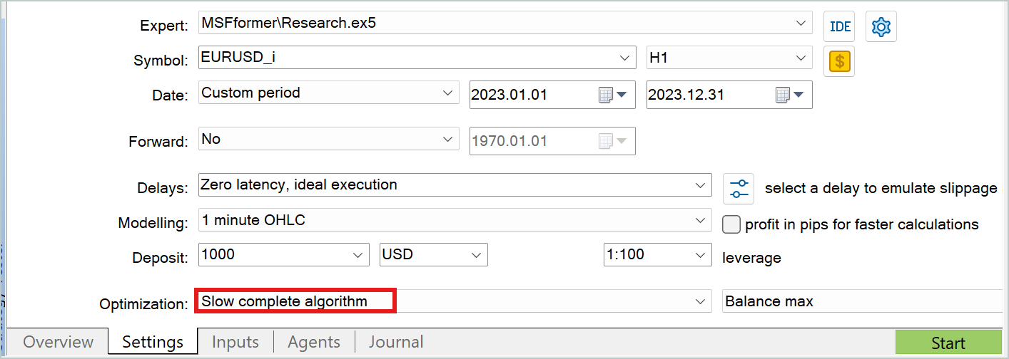
In both cases, it is convenient to use the slow optimization mode of the strategy tester to collect additional data for the training dataset.
I will not go into a detailed discussion of the programs for interacting with the environment. They have already been covered in previous articles within this series. The complete code for all the programs used in this article is included in the attachments, including the code for interacting with the environment for your independent review.
4. Model Training and Testing
After discussing the algorithms of all the programs used for model training, we move on to the process itself. The models will be trained using real historical data for EURUSD with the H1 timeframe. The training period will cover the entire year of 2023.
We collect the initial training set on the specified historical interval, as discussed earlier. On this dataset, we train the Environment State Encoder model. As mentioned before, the Encoder model uses only historical price movement data and the indicators being analyzed during training. It is obvious that the data is identical for all passes over the same historical data interval. Therefore, at this stage, there is no need to refine the training dataset. So, we train the Encoder model on the initial training dataset until we get the desired result.
During the learning process, we monitor the prediction error. We stop the training process when the error no longer decreases, and its fluctuations remain within a small range.
Naturally, we are interested in what the model has learned. Even though our ultimate goal is to train a profitable Actor policy. I still indulged my curiosity and compared the predicted and actual price movements for a randomly selected subset of the training set.
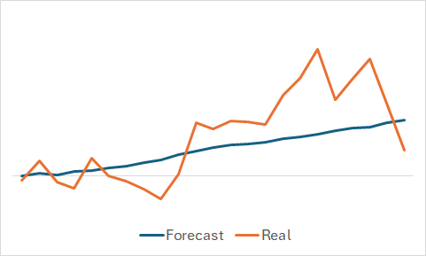
From the graph, it is apparent that the model captured the main trend of the upcoming price movement.
The fairly smooth predicted price movement with minor fluctuations might lead one to believe that the model might have captured the general trend of the training set and would show a similar pattern for all states, regardless of actual data. To confirm or disprove this assumption, we sample another state from the training dataset and perform a similar comparison between the predicted and actual price movements.

Here, we see more significant fluctuations in the predicted values of the price movement. However, they are still relatively close to the actual data.
After training the environmental state Encoder, we proceed to the second stage to train the Actor policy. This process is iterative. The first iteration of training is carried out on the initial training dataset. At this stage, we give the model a preliminary understanding of the environment. Thanks to the profitable runs collected using the Real-ORL method, we establish the basis for our future policy.
During the training process, as in the first stage, we focus on monitoring the models' error. At the initial stage, I would recommend focusing on the Critic's error value. Yes, we need an Actor policy capable of generating profit, but remember our earlier discussion: to train the Actor, we need to train the Critic. Properly establishing dependencies within the Critic will help us adjust the Actor's policy in the right direction.
When the Critic's error stops decreasing and stabilizes, we move to the strategy tester and collect additional data using the Research.mq5 Expert Advisor, which I recommend running in slow optimization mode.
We then continue with the further training of the Actor and Critic models. At the beginning of the retraining process, you may notice a slight increase in the error for both models due to the processing of new data. However, soon you will see a gradual reduction in the error and the achievement of new minima.
Thus, we repeat the iterations of refining the training set and retraining the models.
I would also like to remind you that the architecture of the Actor uses a stochastic head, which introduces some randomness into the actions. Therefore, when testing the trained Actor policy, it is recommended to run multiple passes over a test period. The Actor's policy can be considered trained if the deviations between the passes are negligible.
When preparing this article, we tested the trained model on historical data from January 2024. This period was not part of the training set, so the model encountered new data. The training and test periods are close so we can conclude that the datasets are comparable.
During the training process, I managed to obtain a model that was capable of generating profit on both the training and testing datasets.
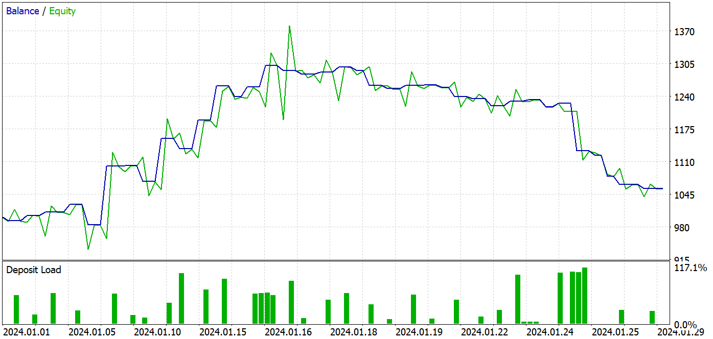
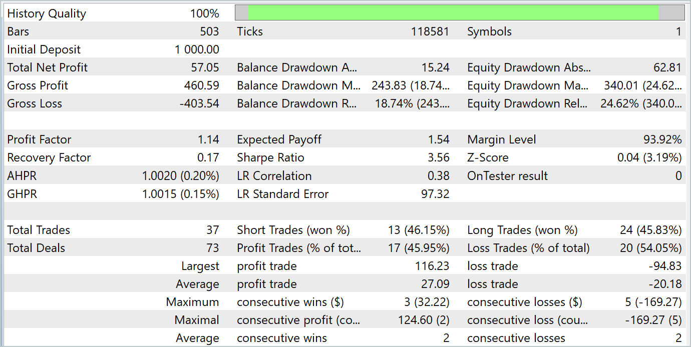
During the testing period, the model made 37 transactions, 17 of which were closed with a profit. This amounted to almost 46%. The share of profitable trades among long and short positions is almost equal. The difference is only 0.32%, which may just be a calculation error due to the small number of transactions. The maximum and average profitable trades are higher than the corresponding metrics for losing trades. This allowed us to close the testing period with a profit. The profit factor was 1.14. However, it is alarming that the profit was made in the first half of the month. It is followed by a lateral movement of the balance. And the last week of the month was marked by a drawdown.
Conclusion
In this article, we trained and tested the model using approaches from the MSFformer method. The results of the testing indicate good performance, suggesting that the proposed approaches are promising. However, the balance drawdown in the last week of the test period is noteworthy, which may indicate the need for additional stages of model training.
References
Programs used in the article
| # | Name | Type | Description |
|---|---|---|---|
| 1 | Research.mq5 | EA | Dataset collecting EA |
| 2 | ResearchRealORL.mq5 | EA | EA for collecting datasets using the Real-ORL method |
| 3 | Study.mq5 | EA | Model training EA |
| 4 | StudyEncoder.mq5 | EA | Encoder training EA |
| 5 | Test.mq5 | EA | Model testing EA |
| 6 | Trajectory.mqh | Class library | System state description structure |
| 7 | NeuroNet.mqh | Class library | A library of classes for creating a neural network |
| 8 | NeuroNet.cl | Code Base | OpenCL program code library |
Translated from Russian by MetaQuotes Ltd.
Original article: https://www.mql5.com/ru/articles/15171
Warning: All rights to these materials are reserved by MetaQuotes Ltd. Copying or reprinting of these materials in whole or in part is prohibited.
This article was written by a user of the site and reflects their personal views. MetaQuotes Ltd is not responsible for the accuracy of the information presented, nor for any consequences resulting from the use of the solutions, strategies or recommendations described.

- Free trading apps
- Over 8,000 signals for copying
- Economic news for exploring financial markets
You agree to website policy and terms of use