Neural Networks Made Easy (Part 91): Frequency Domain Forecasting (FreDF)

Introduction

Forecasting time series of future prices is critical in various financial market scenarios. Most of the methods that currently exist are based on certain autocorrelation in the data. In other words, we exploit the presence of correlation between time steps that exists both in the input data and in the predicted values.

Among the models gaining popularity are those based on the Transformer architecture that use Self-Attention mechanisms for dynamic autocorrelation estimation. Also, we see an increasing interest in the use of frequency analysis in forecasting models. The representation of the sequence of input data in the frequency domain helps avoid the complexity of describing autocorrelation and improves the efficiency of various models.

Another important aspect is the autocorrelation in the sequence of predicted values. Obviously, the predicted values are part of a larger time series, which includes the analyzed and predicted sequences. Therefore, the predicted values preserve the correlation of the analyzed data. But this phenomenon is often ignored in modern forecasting methods. In particular, modern methods predominantly use the Direct Forecast (DF) paradigm, which generates multi-stage forecasts simultaneously. This implicitly assumes the independence of the steps in the sequence of predicted values. This mismatch between model assumptions and data features results in suboptimal forecast quality.

One of the solutions to this problem was proposed in the paper "FreDF: Learning to Forecast in Frequency Domain". The authors of the paper proposed a direct forecast method with frequency gain (FreDF). It clarifies the DF paradigm by aligning the predicted values and the sequence of labels in the frequency domain. When moving to the frequency domain, where the bases are orthogonal and independent, the influence of autocorrelation is effectively reduced. Thus, FreDF combats the inconsistency between the assumption about DF and the existence of autocorrelation of labels, while maintaining the advantages of DF.

The authors of the method tested its effectiveness in a series of experiments, which demonstrated the significant superiority of the proposed approach over modern methods.

1. FreDF Algorithm

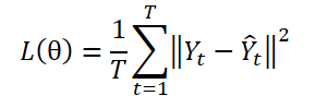
The DF paradigm uses a multiple-output model ɡθ for generating T-step forecasts Ŷ = ɡθ(X). Let Yt be the t-th step of Y, and Yt(n) be the n-th sample observation. The model parameters θ are optimized by minimizing the mean squared error (MSE):

The DF paradigm computes the forecast error at each step independently, treating each element of the sequence as a separate task. However, this approach oversights the autocorrelation present within Y, which contradicts the presence of autocorrelation of labels. As a consequence, this results in a biased likelihood and a deviation from the maximum likelihood principle during model training.

One strategy to overcome this limitation is to represent the sequence of labels in a transformed domain formed by orthogonal bases. In particular, this can be effectively implemented using the Fourier transform, which projects the sequence onto orthogonal bases associated with different frequencies. By transforming the label sequence into the orthogonal frequency domain, it is possible to effectively reduce the dependence on label autocorrelation.

where i is the imaginary unit defined as √(-1),
exp(•) is the Fourier basis associated with the frequency k which is orthogonal for different k values.

Due to the orthogonality of the basis, the frequency domain representation of the label sequence bypasses the dependence arising from autocorrelation in the time domain. This highlights the potential of frequency-domain prediction learning.

With the classical use of DF approaches, at a given time stamp n, the historical sequence Xn is input into the model to generate T-step forecasts, denoted as Ŷn=ɡθ(Xn). The forecast error in the time domain Ltmp is calculated.

In addition to the classical approach, the authors of the FreDF method propose to transform predicted values and label sequences into the frequency domain. Then the prediction error in the frequency domain is calculated using the following formula:

Here each term of the summation is a matrix of complex numbers A; |A| denotes the operation of computing and summing the modulus of each element in the matrix. In this case, the modulus of a complex number a = ar + i ai is computed as √(ar^2 + ai^2).

Please note that due to the different numerical characteristics of the label sequence in the frequency domain, the authors of the FreDF method do not use the squared loss form (MSE), as is typical for time domain loss error calculations. Specifically, different frequency components often have very different magnitudes, with lower frequencies having higher volumes by several orders of magnitude compared to higher frequencies, which makes squared loss methods unstable.

The prediction errors in the time and frequency domains are combined using the coefficient α in the range of values [0,1], which controls the relative strength of the frequency domain equalization:

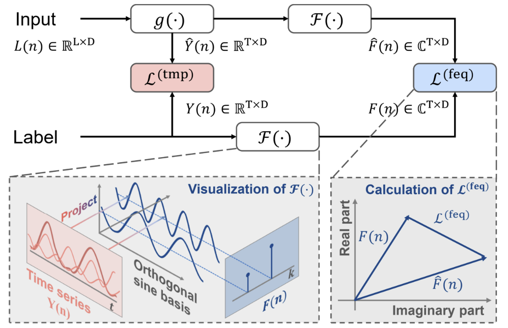
FreDF bypasses the effect of autocorrelation of target values by aligning the generated predicted values and the sequence of labels in the frequency domain. It also preserves the advantages of D.F., such as efficient output and multitasking capabilities. The notable feature of FreDF is its compatibility with various forecasting models and transformations. This flexibility significantly expands the potential scope of FreDF application.

The author's visualization of the method is presented below.

2. Implementing in MQL5

After considering the theoretical aspects of the proposed FreDF method, let's move on to the practical part of our article, in which we will implement our vision of the approach. From the theoretical description presented above, it can be concluded that the proposed approach does not introduce any specific design features into the model architecture. Moreover, it does not affect the actual operation of the model. Its effect can only be seen during the model training process. Probably the proposed FreDF method can be compared to some complex loss function. So, we will use it to train the model whose target labels, according to our a priori knowledge, have autocorrelation dependencies.

Before we begin to build a new object for implementing the proposed approaches, it is worth noting that the authors of the method used the Fourier transform to transform data from a time series to a frequency domain. It must be said that the FreDF method is quite flexible. It also works well in combination with other methods transforming data into the orthogonal domain. The authors of the method conducted a series of experiments to prove its effectiveness when using other transformations. The results of these experiments are presented below.

As can be seen, the models using the Fourier transform show better results.

I would like to draw your attention to the coefficient α. Its value of about 0.8 seems optimal based on the results of the experiments. It should be noted that if forecasting is only performed in the frequency domain (using α equal to 1), according to the results of the same experiments, the model accuracy decreases.

Thus, we can conclude that in order to obtain an optimal time series forecasting model, the training process should include both the time and frequency domains of the signal under study. Different representations allow us to obtain more information about the signal and, as a result, train a more efficient model.

But let's get back to our implementation. According to the results of the experiments conducted by the method authors, the Fourier transform allows training models with a smaller forecast error. In the previous article, we have already implemented the direct and reverse fast Fourier transform. We can use these developments in our new implementation.

To implement the FreDF approaches, we will create a new class CNeuronFreDFOCL, which will inherit the main functionality from the neural layer base class CNeuronBaseOCL. The structure of the new class is shown below.

class CNeuronFreDFOCL   :  public CNeuronBaseOCL
  {
protected:
   uint              iWindow;
   uint              iCount;
   uint              iFFTin;
   bool              bTranspose;
   float             fAlpha;
   //---
   CBufferFloat      cForecastFreRe;
   CBufferFloat      cForecastFreIm;
   CBufferFloat      cTargetFreRe;
   CBufferFloat      cTargetFreIm;
   CBufferFloat      cLossFreRe;
   CBufferFloat      cLossFreIm;
   CBufferFloat      cGradientFreRe;
   CBufferFloat      cGradientFreIm;
   CBufferFloat      cTranspose;
   //---
   virtual bool      FFT(CBufferFloat *inp_re, CBufferFloat *inp_im, 
                         CBufferFloat *out_re, CBufferFloat *out_im, bool reverse = false);
   virtual bool      Transpose(CBufferFloat *inputs, CBufferFloat *outputs, uint rows, uint cols);
   virtual bool      FreqMSA(CBufferFloat *target, CBufferFloat *forecast, CBufferFloat *gradient);
   virtual bool      CumulativeGradient(CBufferFloat *gradient1, CBufferFloat *gradient2, 
                                        CBufferFloat *cummulative, float alpha);
   //---
   virtual bool      feedForward(CNeuronBaseOCL *NeuronOCL);
   virtual bool      updateInputWeights(CNeuronBaseOCL *NeuronOCL)   {  return true;   }
   virtual bool      calcInputGradients(CNeuronBaseOCL *NeuronOCL);

public:
                     CNeuronFreDFOCL(void)   {};
                    ~CNeuronFreDFOCL(void)   {};
   //---
   virtual bool      Init(uint numOutputs, uint myIndex, COpenCLMy *open_cl, 
                          uint window, uint count, float alpha, bool need_transpose = true, 
                          ENUM_OPTIMIZATION optimization_type = ADAM, uint batch = 1);
   virtual bool      calcOutputGradients(CArrayFloat *Target, float &error);
   //---
   virtual bool      Save(int const file_handle);
   virtual bool      Load(int const file_handle);
   //---
   virtual int       Type(void)        const                      {  return defNeuronFreDFOCL; }
   virtual void      SetOpenCL(COpenCLMy *obj);
  };

The presented structure of the new class has two notable features:

• Internal objects are represented only by data buffers and there are no internal layers
• The calcOutputGradients method is overridden

One more implicit feature can be mentioned here: this object does not contain trainable parameters, which is quite rare. All these features are related to the purpose of the class: we are creating a class of a complex loss function, not a trainable neural layer. And the calcOutputGradients method in our neural layer architecture is responsible for calculating the deviations of predicted values from the target ones. We will get acquainted with the purpose of the internal objects and variables while implementing the methods.

All objects are declared statically, allowing us to leave the class constructor and destructor "empty". All operations related to freeing the memory will be performed by the system itself.

Class objects are initialized in the Init method. As usual, in the parameters of this method, we pass the main constants that define the architecture of the class. Here we have:

• a window describing one element of the input data,
• count for the number of elements in the sequence,
• alpha coefficient for the force of equalization of the frequency and time domains,
• the need_transpose flag indicating the need to transpose data for frequency conversion.

This object will be used at the output of the model. Therefore, the input is the predicted values generated by our model. Data must be provided in a format consistent with the target results. The window and count parameters correspond to both predicted and target values. We also provide the user with the ability to transform data into the frequency domain in a different plane. This is why we introduced the need_transpose flag.

I would like to cite here the results of some other experiments conducted by the authors of the method. They tested the performance of the models when comparing frequency characteristics in unitary time series of a multivariate sequence (T), in terms of individual time steps (D) and for the total sequence (2D).

The best results were demonstrated by the model with representing frequency characteristics of the general aggregate sequence. The comparison of frequency characteristics of individual time steps turned out to be the outsider of the experiment. The analysis of frequency characteristics of unitary time series was second best, slightly behind the leader.

In our implementation, we provide the user with the ability to select the measurement for frequency conversion by specifying the corresponding need_transpose flag value. To compare 2-dimensional frequency characteristics, specify the size of the entire sequence in the window parameter and use the following values for the remaining parameters:

• count: 1,
• need_transpose: false.

bool CNeuronFreDFOCL::Init(uint numOutputs, uint myIndex, COpenCLMy *open_cl, 
                           uint window, uint count, float Alpha, bool need_transpose = true, 
                           ENUM_OPTIMIZATION optimization_type = ADAM, uint batch = 1)
  {
   if(!CNeuronBaseOCL::Init(numOutputs, myIndex, open_cl, window * count, optimization_type, batch))
      return false;

In the method body, we first call the relevant parent class method that has the same name and check the result of the operations. Again, the parent class implements the necessary set of controls, including the size of the neural layer being created. For the layer size, we specify the product of variables window and count. Obviously, if you specify a zero value in just one of them, the entire product will be equal to "0", and the parent class method will fail.

After successful execution of the parent class method, we save the obtained values in local variables.

   bTranspose = need_transpose;
   iWindow = window;
   iCount = count;
   fAlpha = MathMax(0, MathMin(Alpha, 1));
   activation = None;

As we have seen earlier, for the fast Fourier transform, we need buffers with a size of a power of 2. Let's calculate the sizes of data buffers:

//--- Calculate FFTsize
   uint size = (bTranspose ? count : window);
   int power = int(MathLog(size) / M_LN2);
   if(MathPow(2, power) != size)
      power++;
   iFFTin = uint(MathPow(2, power));

The next step is to initialize the internal data buffers. First, we initialize the frequency response buffers of the predicted values. We use a 2 data buffer design. One buffer is used for recording data of the real component, and the second one is used for the imaginary one.

//---
   uint n = (bTranspose ? iWindow : iCount);
   if(!cForecastFreRe.BufferInit(iFFTin * n, 0) || !cForecastFreRe.BufferCreate(OpenCL))
      return false;
   if(!cForecastFreIm.BufferInit(iFFTin * n, 0) || !cForecastFreIm.BufferCreate(OpenCL))
      return false;

Next, we create similar buffers for the frequency characteristics of the target values:

   if(!cTargetFreRe.BufferInit(iFFTin * n, 0) || !cTargetFreRe.BufferCreate(OpenCL))
      return false;
   if(!cTargetFreIm.BufferInit(iFFTin * n, 0) || !cTargetFreIm.BufferCreate(OpenCL))
      return false;

We write the prediction error into buffers cLossFreeRe and cLossFree:

   if(!cLossFreRe.BufferInit(iFFTin * n, 0) || !cLossFreRe.BufferCreate(OpenCL))
      return false;
   if(!cLossFreIm.BufferInit(iFFTin * n, 0) || !cLossFreIm.BufferCreate(OpenCL))
      return false;

Please note the importance of comparing both components of the frequency characteristics. For correct forecasting of time series, both the amplitudes and phases of the frequency characteristics of the time series are important.

It is also necessary to create buffers for recording error gradients at the level of predicted time series values:

   if(!cGradientFreRe.BufferInit(iFFTin * n, 0) || !cGradientFreRe.BufferCreate(OpenCL))
      return false;
   if(!cGradientFreIm.BufferInit(iFFTin * n, 0) || !cGradientFreIm.BufferCreate(OpenCL))
      return false;

In order to save memory, we can exclude buffers cGradientFreeRe and cGradientFreeIm. They can be easily replaced, for example, with buffers cForecastFreeRe and cForecastFreeIm. But their presence makes the code more readable. Also, the amount of memory they use in our case is not critical.

Finally, we will create a temporary buffer to write the transposed values, if required:

      if(!cTranspose.BufferInit(iWindow * iCount, 0) || !cTranspose.BufferCreate(OpenCL))
         return false;
//---
   return true;
  }

After data initialization, we usually create a feed-forward pass method. It was already said above that an object of this class does not perform operations with data during operation. As you know, the feed-forward method describes the model's operating mode. We could redefine the feed-forward pass method with a "dummy", but then how would we transfer data? As always, we would like to minimize the data copying process, because the data volume can be different, and process organization adds "overhead costs". In this context, we make the feed-forward pass method as simple as possible. In this method, we only check the correspondence of pointers to result buffers in the current and previous layers. If necessary, we replace the pointer in the current layer with the result buffer of the previous layer.

bool CNeuronFreDFOCL::feedForward(CNeuronBaseOCL *NeuronOCL)
  {
   if(!NeuronOCL || !NeuronOCL.getOutput())
      return false;
   if(NeuronOCL.getOutput() != Output)
     {
      Output.BufferFree();
      delete Output;
      Output = NeuronOCL.getOutput();
     }
//---
   return true;
  }

Thus, we replace the pointer to one buffer instead of transferring data regardless of its volume. Please note that control is performed on each pass, and the data buffers are replaced only on the first one.

We implement the main functionality of the class for the backpropagation pass. Let's first do a little preparatory work. To fully implement the required functionality, we will create 2 small kernels on the OpenCL program side.

Authors of the FreDF method recommend using MAE as a loss function when estimating deviations in the frequency domain. They also note a decrease in the training stability when using MSE. Let me remind you that our basic neural layer class CNeuronBaseOCL uses exactly MSE to determine the error gradient. So, we need to create a kernel to determine the forecast error gradient using MAE. From a mathematical point of view, this is quite simple: we just need to subtract the vector of predicted values from the vector of target labels.

__kernel void GradientMSA(__global float *matrix_t,
                          __global float *matrix_o,
                          __global float *matrix_g
                         )
  {
   int i = get_global_id(0);
   matrix_g[i] = matrix_t[i] - matrix_o[i];
  }

After determining the error gradient in the frequency and time domains, we need to combine the error gradients using the temperature coefficient. Let's implement this functionality in the CumulativeGradient kernel, which should be quite easy to understand, I think.

__kernel void CumulativeGradient(__global float *gradient_freq,
                                 __global float *gradient_tmp,
                                 __global float *gradient_out,
                                 float alpha
                                )
  {
   int i = get_global_id(0);
   gradient_out[i] = alpha * gradient_freq[i] + (1 - alpha) * gradient_tmp[i];
  }

Let me remind you that to transform data from the time domain to the frequency domain and back, we will use the fast Fourier transform algorithm, which we implemented in the previous article. That article provides a description of the algorithm used and the method for placing the kernel in the execution queue.

Now we will not consider the algorithms for methods of placing kernels in the execution queue. They all follow the same procedure, which has already been presented several times in the articles within this series, including the previous one.

Let's consider the CNeuronFreDFOCL::calcOutputGradients method, which implements the main functionality of our class. As you know, according to the structure of our models, this method determines the deviation of the predicted values from the target labels. In the method parameters, we receive a pointer to the buffer with target values. After performing the method operations, we need to save the error gradient into the corresponding buffer of the current layer.

bool CNeuronFreDFOCL::calcOutputGradients(CArrayFloat *Target, float &error)
  {
   if(!Target)
      return false;
   if(Target.Total() < Output.Total())
      return false;

In the method body, we check the correctness of the received pointer to the target value buffer. Also, its size must be no less than the model's result tensor.

Since the received buffer may not have a copy of itself on the OpenCL context side, we have to create it there for subsequent calculations. However, for more economical use of OpenCL context resources, we will transfer the obtained data to the already created gradient buffer.

   if(Target.Total() == Output.Total())
     {
      if(!Gradient.AssignArray(Target))
         return false;
     }
   else
     {
      for(int i = 0; i < Output.Total(); i++)
        {
         if(!Gradient.Update(i, Target.At(i)))
            return false;
        }
     }
   if(!Gradient.BufferWrite())
      return false;

Here there are 2 possible developments. If the sizes of the target label and predicted value buffers are equal, then we use the existing copy method. Otherwise, we use a loop to transfer the required number of values. In any case, after copying the data, we transfer it to the OpenCL context memory.

The obtained data is then used to calculate deviations in both the time and frequency domains. Please paying attention that when calculating deviations in the time domain, the error gradient buffer of our layer will be overwritten by the calculated deviations, while the obtained target values will be completely lost. Therefore, before calculating the deviations in the time domain, we at least need to decompose the obtained time series of target labels into frequency components.

A time series can be decomposed into frequency characteristics in two dimensions. The one to be used is determined by the value of the bTranspose flag. If the flag is set to true, we first transpose the model's result buffer and then decompose it into frequency responses:

   if(bTranspose)
     {
      if(!Transpose(Output, GetPointer(cTranspose), iWindow, iCount))
         return false;
      if(!FFT(GetPointer(cTranspose), NULL, GetPointer(cForecastFreRe), GetPointer(cForecastFreIm), false))
         return false;

We perform similar operations for the target label tensor:

      if(!Transpose(Gradient, GetPointer(cTranspose), iWindow, iCount))
         return false;
      if(!FFT(GetPointer(cTranspose), NULL, GetPointer(cTargetFreRe), GetPointer(cTargetFreIm), false))
         return false;
     }

If the bTranspose flag value is false, then we perform the decomposition of the target and predicted values into the corresponding frequency characteristics without preliminary transposition:

   else
     {
      if(!FFT(Output, NULL, GetPointer(cForecastFreRe), GetPointer(cForecastFreIm), false))
         return false;
      if(!FFT(Gradient, NULL, GetPointer(cTargetFreRe), GetPointer(cTargetFreIm), false))
         return false;
     }

Once the frequency characteristics are determined, we can calculate deviations in both the time and frequency domains without worrying about losing target values.

   if(!FreqMSA(GetPointer(cTargetFreRe), GetPointer(cForecastFreRe), GetPointer(cLossFreRe)))
      return false;
   if(!FreqMSA(GetPointer(cTargetFreIm), GetPointer(cForecastFreIm), GetPointer(cLossFreIm)))
      return false;
   if(!FreqMSA(Gradient, Output, Gradient))
      return false;

Note that in the frequency domain, we determine deviations in both the real and imaginary parts of the frequency response. Because the value of the phase shift is no less important than the signal amplitude. However, we cannot directly approximate the gradients of time and frequency domain errors. Obviously, the data is incomparable. Therefore, we first need to return the gradients of the frequency response error to the time domain. For this, we will use the inverse Fourier transform.

   if(!FFT(GetPointer(cLossFreRe), GetPointer(cLossFreIm), GetPointer(cGradientFreRe), GetPointer(cGradientFreIm), true))
      return false;

The error gradients of the time and frequency domains have been brought into a comparable form. Now, the measurement of frequency characteristic extraction depends on the value of the bTranspose flag. Therefore, we need to transform the frequency domain error gradient according to the flag value. Only then can we determine the cumulative error gradient of our model.

   if(bTranspose)
     {
      if(!Transpose(GetPointer(cGradientFreRe), GetPointer(cTranspose), iCount, iWindow))
         return false;
      if(!CumulativeGradient(GetPointer(cTranspose), Gradient, Gradient, fAlpha))
         return false;
     }
   else
      if(!CumulativeGradient(GetPointer(cGradientFreRe), Gradient, Gradient, fAlpha))
         return false;
//---
   return true;
  }

Do not forget to control the results at each step. The logical value of the operations is returned to the caller.

After determining the error gradient at the model output, we need to pass it to the previous layer. We implement this functionality in the CNeuronFreDFOCL::calcInputGradients method, which receives a pointer to the object of the previous neural layer in its parameters.

Remember that our layer does not contain trainable parameters. During the feed-forward pass, we have replaced the data buffer and are showing the values from the previous layer as the results. What is the purpose of this method? It is very simple. We just need to adjust the cumulative error gradient calculated above to the activation function of the previous layer.

bool CNeuronFreDFOCL::calcInputGradients(CNeuronBaseOCL *NeuronOCL)
  {
   if(!NeuronOCL)
      return false;
//---
   return DeActivation(NeuronOCL.getOutput(), NeuronOCL.getGradient(), Gradient, NeuronOCL.Activation());
  }

Since our class does not contain trainable parameters, we redefine the updateInputWeights method with an "empty stub".

The absence of tranable parameters in the class also influence file operation methods. Because we don't need to store irrelevant internal objects. Therefore, when saving data, we only call the parent class method of the same name.

bool CNeuronFreDFOCL::Save(const int file_handle)
  {
   if(!CNeuronBaseOCL::Save(file_handle))
      return false;

We save the values of the variables describing the design features of the object:

   if(FileWriteInteger(file_handle, int(iWindow)) < INT_VALUE)
      return false;
   if(FileWriteInteger(file_handle, int(iCount)) < INT_VALUE)
      return false;
   if(FileWriteInteger(file_handle, int(iFFTin)) < INT_VALUE)
      return false;
   if(FileWriteInteger(file_handle, int(bTranspose)) < INT_VALUE)
      return false;
   if(FileWriteFloat(file_handle, fAlpha) < sizeof(float))
      return false;
//---
   return true;
  }

The Load algorithm for restoring an object from a data file looks a little more complicated. Here we first restore the elements of the parent class:

bool CNeuronFreDFOCL::Load(const int file_handle)
  {
   if(!CNeuronBaseOCL::Load(file_handle))
      return false;

Then we load the variable data in the order they are saved, remembering to check when the end of the data file is reached:

   if(FileIsEnding(file_handle))
      return false;
   iWindow = uint(FileReadInteger(file_handle));
   if(FileIsEnding(file_handle))
      return false;
   iCount = uint(FileReadInteger(file_handle));
   if(FileIsEnding(file_handle))
      return false;
   iFFTin = uint(FileReadInteger(file_handle));
   if(FileIsEnding(file_handle))
      return false;
   bTranspose = bool(FileReadInteger(file_handle));
   if(FileIsEnding(file_handle))
      return false;
   fAlpha = FileReadFloat(file_handle);

Then we need to initialize the nested objects in accordance with the loaded parameters of the class architecture. Object are initialized similarly to the algorithm for initializing a new class instance:

   uint n = (bTranspose ? iWindow : iCount);
   if(!cForecastFreRe.BufferInit(iFFTin * n, 0) || !cForecastFreRe.BufferCreate(OpenCL))
      return false;
   if(!cForecastFreIm.BufferInit(iFFTin * n, 0) || !cForecastFreIm.BufferCreate(OpenCL))
      return false;
   if(!cTargetFreRe.BufferInit(iFFTin * n, 0) || !cTargetFreRe.BufferCreate(OpenCL))
      return false;
   if(!cTargetFreIm.BufferInit(iFFTin * n, 0) || !cTargetFreIm.BufferCreate(OpenCL))
      return false;
   if(!cLossFreRe.BufferInit(iFFTin * n, 0) || !cLossFreRe.BufferCreate(OpenCL))
      return false;
   if(!cLossFreIm.BufferInit(iFFTin * n, 0) || !cLossFreIm.BufferCreate(OpenCL))
      return false;
   if(!cGradientFreRe.BufferInit(iFFTin * n, 0) || !cGradientFreRe.BufferCreate(OpenCL))
      return false;
   if(!cGradientFreIm.BufferInit(iFFTin * n, 0) || !cGradientFreIm.BufferCreate(OpenCL))
      return false;
   if(bTranspose)
     {
      if(!cTranspose.BufferInit(iWindow * iCount, 0) || !cTranspose.BufferCreate(OpenCL))
         return false;
     }
   else
     {
      cTranspose.BufferFree();
      cTranspose.Clear();
     }
//---
   return true;
  }

This concludes the description of the methods of our new CNeuronFreDFOCL class. You can see the full code of this class in the attachment.

After constructing the methods of the new class, we usually move on to describing the trainable model architecture. But in this article, we have built a rather unusual neural layer. We have implemented a complex loss function in the form of a neural layer. So, we can add the above created object to one of the models we trained earlier, retrain it and see how the results change. For my experiments I chose the FEDformer model; its architecture is described here. Let's add a new layer to it.

bool CreateEncoderDescriptions(CArrayObj *encoder)
  {
//---
........
........
//--- layer 17
   if(!(descr = new CLayerDescription()))
      return false;
   descr.type = defNeuronFreDFOCL;
   descr.window = BarDescr;
   descr.count =  NForecast;
   descr.step = int(true);
   descr.probability = 0.8f;
   descr.activation = None;
   descr.optimization = ADAM;
   if(!encoder.Add(descr))
     {
      delete descr;
      return false;
     }
//---
   return true;
  }

After thinking about it for a while, I decided to expand the experiment. The authors of the FreDF method proposed their own algorithm for using the dependencies in predicted results. Actually, there is also a dependence between the individual parameters of our Actor's results. For example, the volumes of buy and sell trades are mutually exclusive, because at any given time we only have an open position in one direction. Stop loss and take profit parameters determine the strength of the most likely upcoming move. Therefore, the take profit of a long position should be correlated to some extent with the stop loss of a short position and vice versa. Similar reasoning can be used to suggest dependencies in the predicted Critic values. So why not extend the experiment to the models mentioned? No sooner said than done. Adding a new layer to the Actor and Critic models:

bool CreateDescriptions(CArrayObj *actor, CArrayObj *critic)
  {
//---
   CLayerDescription *descr;
//---
   if(!actor)
     {
      actor = new CArrayObj();
      if(!actor)
         return false;
     }
   if(!critic)
     {
      critic = new CArrayObj();
      if(!critic)
         return false;
     }
//--- Actor
.........
.........
//--- layer 17
   if(!(descr = new CLayerDescription()))
      return false;
   descr.type = defNeuronFreDFOCL;
   descr.window = NActions;
   descr.count =  1;
   descr.step = int(false);
   descr.probability = 0.8f;
   descr.activation = None;
   descr.optimization = ADAM;
   if(!actor.Add(descr))
     {
      delete descr;
      return false;
     }
//--- Critic
.........
.........
//--- layer 17
   if(!(descr = new CLayerDescription()))
      return false;
   descr.type = defNeuronFreDFOCL;
   descr.window = NRewards;
   descr.count =  1;
   descr.step = int(false);
   descr.probability = 0.8f;
   descr.activation = None;
   descr.optimization = ADAM;
   if(!critic.Add(descr))
     {
      delete descr;
      return false;
     }
//---
   return true;
  }

Please note that in this case we are analyzing the frequency characteristics of the entire sequence of results, and not of individual unitary series.

Our implementation of the approaches proposed by the FreDF method does not require any adjustments to the Expert Advisors used for model training and interaction with the environment. This means that to test the obtained results, we can use previously prepared Expert Advisors and training datasets.   

3. Testing

We have done quite a lot of work to implement the approaches proposed by the authors of FreDF using MQL5. Now we move on to the final stage of our work: training and testing.

As mentioned above, we will train the models using the previously created Expert Advisor and pre-collected training data. In our articles, we train models on the historical data of the EURUSD instrument with the H1 timeframe for year 2023.

First we train the model of the environment state Encoder. The model is trained to predict future states of the environment over a planning horizon determined by the NForecast constant. In my experiment, I used 12 subsequent candles. The forecast is generated in the context of all analyzed parameters describing the state of the environment.

#define        NForecast               12            //Number of forecast

In the process of Encoder training, we can see a reduction in the forecast error compared to a similar model without using FreDF approaches. However, we did not perform a graphical comparison of the forecast results. Therefore, it is difficult to judge the actual quality of the forecast values. It should be noted here that, as strange as it may seem, our goal is not to obtain the most accurate forecasts of all the analyzed indicators. The Actor model uses Encoder's latent space to decide on optimal actions. The goal of the first stage of training is to obtain the most informative latent space of the Encoder, which would encode the most likely upcoming price movement.

As before, the Encoder model analyzes only price movement, so during the first stage of training we do not need to update the training set.

In the second stage of our learning process, we search for the most optimal Actor action policy. Here we run iterative training of Actor and Critic models, which alternates with updating the training dataset.

As a result of several iterations of Actor policy training, we managed to get a model that can generate profit. We tested the performance of the trained model in the MetaTrader 5 strategy tester using real historical data for January 2024. The testing parameters fully corresponded to the parameters of the training dataset, including the instrument, timeframe and parameters of the analyzed indicators. The test results are presented in the screenshots below. 

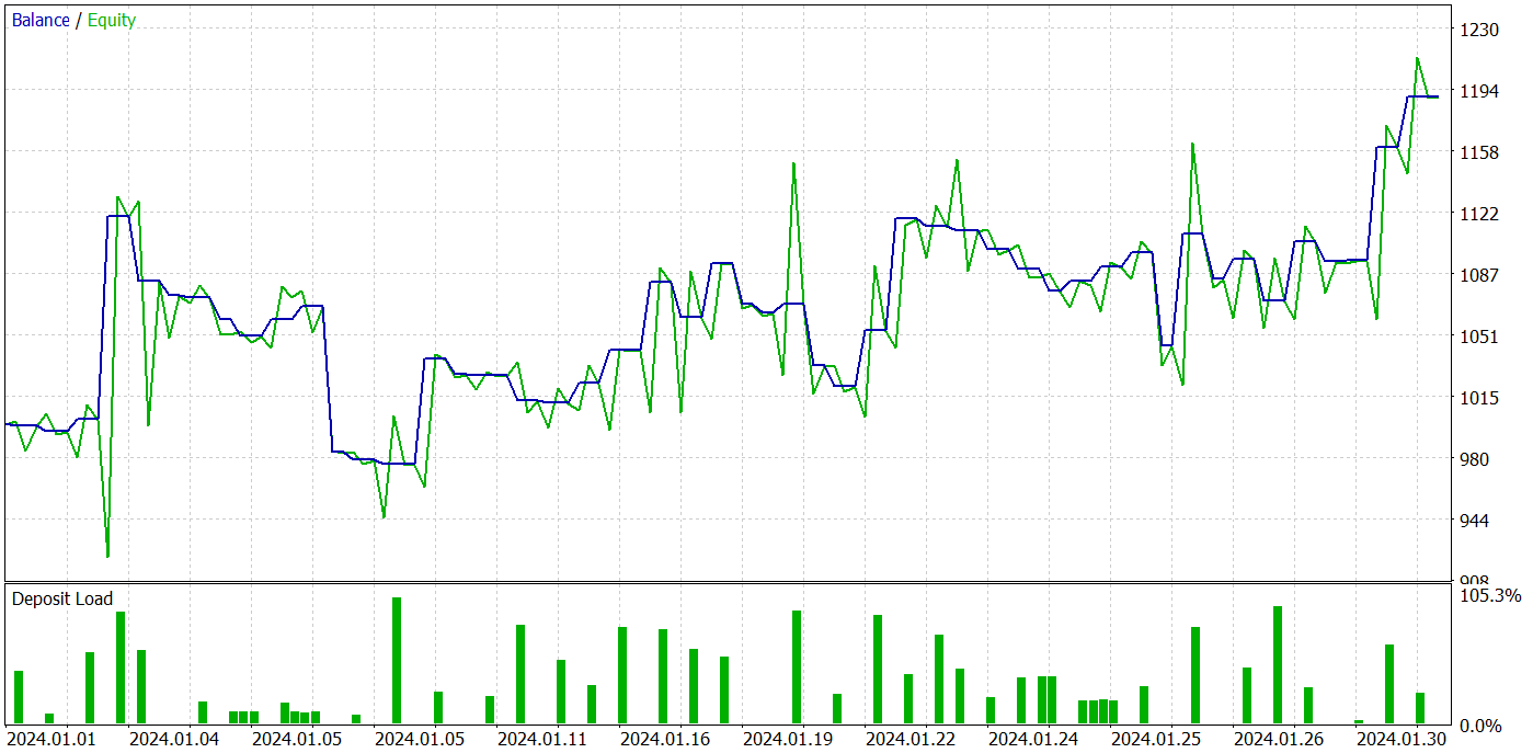
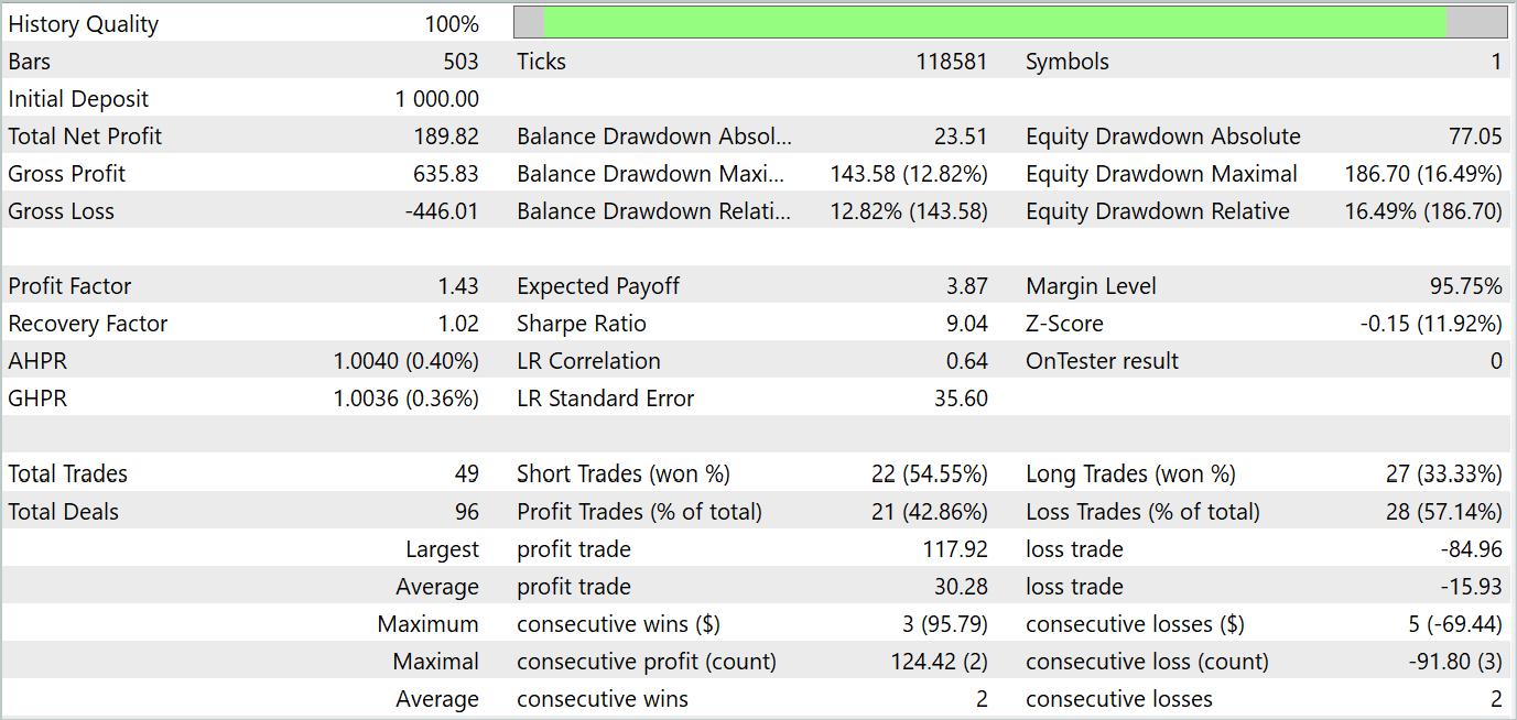
Based on the testing results, we can notice a clear trend towards an increase in the account balance. During the testing period, the model executed 49 trades, 21 of which were closed with a profit. Yes, less than half of the positions were profitable. However, the average profitable trade is almost 2 times larger than the average losing trade. As a result, the profit factor of the model on the test dataset is 1.43 and the total income for the month is about 19%.

Conclusion

In this article, we discussed the FreDF method, which aims to improve time series forecasting. The authors of the method empirically substantiated that ignoring autocorrelation in the labeled sequence leads to a bias in the likelihood and a deterioration in the quality of forecasts in the current DF paradigm. They presented a simple but effective modification of the current DF paradigm, which takes into account autocorrelation by aligning forecast and label sequences in the frequency domain. The FreDF method is compatible with various forecasting models and transformations, making it flexible and versatile.

In the practical part of the article, we implemented our vision of the proposed approaches in the MQL5 language. We supplemented the previously created FEDformer model with proposed approaches and conducted training. Then we tested the trained model. The testing results suggest the effectiveness of the proposed approaches, since the addition of FreDF had increased the efficiency of the model, all other things being equal.

I would like to note the flexibility of the FreDF method, which allows it to be used effectively with a wide range of existing models.

References

• FreDF: Learning to Forecast in Frequency Domain
• Other articles from this series

Programs used in the article

#	Name	Type	Description
1	Research.mq5	Expert Advisor	Example collection EA
2	ResearchRealORL.mq5	Expert Advisor	EA for collecting examples using the Real-ORL method
3	Study.mq5	Expert Advisor	Model training EA
4	StudyEncoder.mq5	Expert Advisor	Encode Training EA
5	Test.mq5	Expert Advisor	Model testing EA
6	Trajectory.mqh	Class library	System state description structure
7	NeuroNet.mqh	Class library	A library of classes for creating a neural network
8	NeuroNet.cl	Code Base	OpenCL program code library