
Neural Networks Made Easy (Part 95): Reducing Memory Consumption in Transformer Models

Introduction
The introduction of the Transformer architecture back in 2017 led to the emergence of Large Language Models (LLMs), which demonstrate high results in solving natural language processing problems. Quite soon the advantages of Self-Attention approaches have been adopted by researchers in virtually every area of machine learning.
However, due to its autoregressive nature, the Transformer Decoder is limited by the memory bandwidth used to load and store the Key and Value entities at each time step (known as KV caching). Since this cache scales linearly with model size, batch size, and context length, it can even exceed the memory usage of the model weights.
This problem is not new. There are different approaches to solving it. The most widely used methods imply direct reduction of the KV heads used. In 2019, the authors of the paper Fast Transformer Decoding: One Write-Head is All You Need proposed the Multi-Query Attention (MQA) algorithm, which uses only one Key and Value projection for all attention heads at the level of one layer. This reduces memory consumption for KV cache by 1/heads. This significant reduction in resource consumption leads to some degradation in the model quality and stability.
The authors of the Grouped-Query Attention (GQA) method, described in the paper GQA: Training Generalized Multi-Query Transformer Models from Multi-Head Checkpoints (2023), presented an intermediate solution for separating multiple KV heads into several attention groups. KV cache size reduction efficiency when using GQA equals groups/heads. With a reasonable number of heads, GQA can achieve near parity with the base model in various tests. However, the KV cache size reduction is still limited to 1/heads when using MQA. This may not be enough for some applications.
To go beyond this limitation, the authors of the paper MLKV: Multi-Layer Key-Value Heads for Memory Efficient Transformer Decoding proposed a multi-level Key and Value sharing algorithm (MLKV). They take sharing use of KV one step further. MLKV not only divides KV heads between the attention heads of one layer, but also between the attention heads of other levels. KV heads can be used for attention head groups in one layer and/or for attention head groups in subsequent layers. In extreme cases, one KV head can be used for all attention heads of all layers. The authors of the method experiment with various configurations, which they use as grouped Query both at the same level and between different levels. Even with configurations in which the number of KV heads are fewer than layers. The experiments presented in this paper demonstrate that these configurations provide a reasonable trade-off between performance and achieved memory savings. Practical reduction of memory usage to 2/layers of the original KV cache size does not lead to a significant deterioration in the quality of the model.
1. MLKV Method
The MLKV method is a logical continuation of the MQA and GQA algorithms. In the specified methods, the KV cache size is reduced due to the reduction of KV heads, which are shared by a group of attention heads within a single Self-Attention layer. A completely expected step is the sharing of Key and Value entities between Self-Attention layers. This step may be justified by recent research into the role of the FeedForward block in the algorithmTransformer. It is assumed that the specified block simulates the "Key-Value" memory, processing different levels of information. However, what is most interesting for us is the observation that groups of successive layers compute similar things. More precisely, the lower levels deal with superficial patterns, and the upper levels deal with more semantic details. Thus, it can be concluded that attention can be delegated to groups of layers while keeping the necessary computations in the FeedForward block. Intuitively, KV heads can be shared between layers that have similar targets.
Developing these ideas, the authors of the MLKV method offer multi-level key exchange. MLKV not only shares KV heads among Query attention heads in the same Self-Attention layer, but also among the attention heads in other layers. This allows the reduction of the total number of KV heads in the Transformer, thus allowing for an even smaller KV cache.
MLKV can be written as follows:
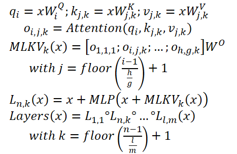
Below is the author's visualization of the comparison of KV cache size reduction methods.

Experiments conducted by the authors of the method demonstrate a clear trade-off between memory and accuracy. Designers are left to choose what to sacrifice. Furthermore, there are many factors to consider. For the number of KV heads greater than or equal to the number of layers, it is still better to use GQA/MQA instead of MLKV. The authors of the method assume that the presence of multiple KV heads in multiple layers is more important than having multiple KV heads in one layer. In other words, you should sacrifice KV heads at the layer level first (GQA/MQA) and cross-layer second (MLKV).
For more memory intensive situations requiring the number of KV heads less than the number of layers, the only way is MLKV. This design solution is viable. The authors of the method found that when the attention heads are reduced to being less than a half of the number of layers, MLKV works very close to MQA. This means it should be a relatively simple solution if you need the KV cache to be half the size provided by MQA.
If a lower value is required, we can use the number of KV heads up to 6 times less than the number of layers without a sharp deterioration in quality. Anything below that becomes questionable.
2. Implementing in MQL5
We have briefly considered the theoretical description of the proposed approaches. Now, we can move on to their practical implementation using MQL5. Here we will implement the MLKV method. In my opinion, this is a more general approach, while MQA and GQA can be presented as special cases of MLKV.
The most acute issue of the upcoming implementation is how to transfer information between neural layers. In this case, I decided not to complicate the existing algorithm of how data is exchanged between neural layer objects. Instead, we will use a multilayer sequence block, which we have already implemented many times. We will use CNeuronMLMHAttentionOCL as a parent class for the upcoming implementation.
2.1 Implementing on the OpenCL side
Let's start by preparing kernels on the OpenCL program side. Note that in the selected parent class, we used one concatenated tensor for the parallel generation of the Query, Key and Value entities. The entire mechanism of attention was built on this. However, since we use different numbers of heads for Query and Key-Value, as well as use Key-Value from another level, we should think about dividing the said entities into 2 separate tensors. We have already done something similar when constructing cross-attention blocks.
It means we can take advantage of the existing code and slightly adjust the cross-attention kernel algorithm. We just need to add another kernel parameter indicating the number of KVheads (highlighted in red in the code).
__kernel void MH2AttentionOut(__global float *q,     ///<[in] Matrix of Querys
                              __global float *kv,    ///<[in] Matrix of Keys
                              __global float *score, ///<[out] Matrix of Scores
                              __global float *out, ///<[out] Matrix of attention
                              int dimension,        ///< Dimension of Key
                              int heads_kv
                             )
In the kernel body, to determine the KV head being analyzed, we need to take the remainder from dividing the current attention head by the total number of KV heads.
const int h_kv = h % heads_kv;
Add a shift adjustment in the Key-Value tensor buffer.
   const int shift_k = 2 * dimension * (k + h_kv);
   const int shift_v = 2 * dimension * (k + heads_kv + h_kv);
Further kernel code remains unchanged. Similar edits were made to the backpropagation kernel code MH2AttentionInsideGradients. The full code of these kernels is available in the attachment.
This concludes our work on the OpenCL side. Let's move on to the main program side. Here we first need to restore the functionality of the previously created code. Because an additional parameter in the kernels specified above will lead to errors when calling them. So let's find all calls to these kernels and add the data transfer to a new parameter.
Let me remind you that previously we used the same number of goals for Query and Key-Value.
   if(!OpenCL.SetArgument(def_k_MH2AttentionOut, def_k_mh2ao_heads_kv, (int)iHeads))
     {
      printf("Error of set parameter kernel %s: %d; line %d", __FUNCTION__, GetLastError(), __LINE__);
      return false;
     }
   if(!OpenCL.SetArgument(def_k_MH2AttentionInsideGradients, def_k_mh2aig_heads_kv, (int)iHeads))
     {
      printf("Error of set parameter kernel %s: %d; line %d", __FUNCTION__, GetLastError(), __LINE__);
      return false;
     }
2.2 Creating the MLKV class
Let's continue our project. In the next step, we will create a multilayer attention block class using the MLKV approaches: CNeuronMLMHAttentionMLKV. As mentioned earlier, the new class will be a direct child of the CNeuronMLMHAttentionOCL class. The structure of the new class is shown below.
class CNeuronMLMHAttentionMLKV :  public CNeuronMLMHAttentionOCL
  {
protected:
   uint              iLayersToOneKV;
   uint              iHeadsKV;
   CCollection       KV_Tensors;
   CCollection       KV_Weights;
   CBufferFloat      Temp;
   //---
   virtual bool      feedForward(CNeuronBaseOCL *NeuronOCL);
   virtual bool      AttentionOut(CBufferFloat *q, CBufferFloat *kv, CBufferFloat *scores, CBufferFloat *out);
   virtual bool      AttentionInsideGradients(CBufferFloat *q, CBufferFloat *q_g,
                                              CBufferFloat *kv, CBufferFloat *kv_g,
                                              CBufferFloat *scores, CBufferFloat *gradient);
   //---
   virtual bool      calcInputGradients(CNeuronBaseOCL *prevLayer);
   virtual bool      updateInputWeights(CNeuronBaseOCL *NeuronOCL);

public:
                     CNeuronMLMHAttentionMLKV(void) {};
                    ~CNeuronMLMHAttentionMLKV(void) {};
   virtual bool      Init(uint numOutputs, uint myIndex, COpenCLMy *open_cl,
                          uint window, uint window_key, uint heads, uint heads_kv, uint units_count,
                          uint layers, uint layers_to_one_kv,
                          ENUM_OPTIMIZATION optimization_type, uint batch);
   //---
   virtual int       Type(void)   const   {  return defNeuronMLMHAttentionMLKV;   }
   //---
   virtual bool      Save(int const file_handle);
   virtual bool      Load(int const file_handle);
   virtual bool      WeightsUpdate(CNeuronBaseOCL *source, float tau);
   virtual void      SetOpenCL(COpenCLMy *obj);
  };
As you can see, in the presented class structure we have introduce 2 variables to store the number of KV heads (iHeadsKV) and the frequency of Key-Value tensor update (iLayersToOneKV).
We have also added Key-Value tensor storage collections and weight matrices for their formation (KV_Tensors and KV_Weights respectively).
In addition, we have added a Temp buffer to record intermediate values of error gradients.
The set of class methods is quite standard and I think you already understand their purpose. We will consider them in more detail during the implementation process.
We declare all internal objects as static and thus we can leave the class constructor and destructor empty. Initialization of all nested objects and variables is performed in the Init method. As usual, the parameters of this method contain all the information necessary to create the required object.
bool CNeuronMLMHAttentionMLKV::Init(uint numOutputs, uint myIndex, COpenCLMy *open_cl,
                                    uint window, uint window_key, uint heads, uint heads_kv,


                                    uint units_count, uint layers, uint layers_to_one_kv,
                                    ENUM_OPTIMIZATION optimization_type, uint batch)
  {
   if(!CNeuronBaseOCL::Init(numOutputs, myIndex, open_cl, window * units_count, optimization_type, batch))
      return false;
In the body of the method, we immediately call the relevant method of the base class of all neural layers CNeuronBaseOCL.
Note that we are accessing the base class object, not the direct parent class. This is related to the separation of Query, Key and Value entities into 2 tensors, which leads to a change in the sizes of some data buffers. However, this approach forces us to initialize not only new objects, but also those inherited from the parent class.
After successful execution of the base class initialization method, we save the received class parameters into internal variables.
   iWindow = fmax(window, 1);
   iWindowKey = fmax(window_key, 1);
   iUnits = fmax(units_count, 1);
   iHeads = fmax(heads, 1);
   iLayers = fmax(layers, 1);
   iHeadsKV = fmax(heads_kv, 1);
   iLayersToOneKV = fmax(layers_to_one_kv, 1);
The next step is to calculate the sizes of all buffers to be created.
   uint num_q = iWindowKey * iHeads * iUnits;               //Size of Q tensor
   uint num_kv = 2 * iWindowKey * iHeadsKV * iUnits;        //Size of KV tensor
   uint q_weights = (iWindow + 1) * iWindowKey * iHeads;    //Size of weights' matrix of Q tenzor
   uint kv_weights = 2 * (iWindow + 1) * iWindowKey * iHeadsKV; //Size of weights' matrix of KV tenzor
   uint scores = iUnits * iUnits * iHeads;                  //Size of Score tensor
   uint mh_out = iWindowKey * iHeads * iUnits;              //Size of multi-heads self-attention
   uint out = iWindow * iUnits;                             //Size of out tensore
   uint w0 = (iWindowKey + 1) * iHeads * iWindow;           //Size W0 tensor
   uint ff_1 = 4 * (iWindow + 1) * iWindow;                 //Size of weights' matrix 1-st feed forward layer
   uint ff_2 = (4 * iWindow + 1) * iWindow;                 //Size of weights' matrix 2-nd feed forward layer
Next, we add a loop with a number of iterations equal to the number of internal layers in the attention block being created.
   for(uint i = 0; i < iLayers; i++)
     {
In the body of the loop, we create another nested loop in which we first create buffers to store data. At the second iteration of the nested loop, we will create buffers for recording the corresponding error gradients.
      CBufferFloat *temp = NULL;
      for(int d = 0; d < 2; d++)
        {
         //--- Initilize Q tensor
         temp = new CBufferFloat();
         if(CheckPointer(temp) == POINTER_INVALID)
            return false;
         if(!temp.BufferInit(num_q, 0))
            return false;
         if(!temp.BufferCreate(OpenCL))
            return false;
         if(!QKV_Tensors.Add(temp))
            return false;
Here we first create Query entity tensors. Then we create the relevant tensors for recording Key-Value entities. However, the latter should be created once per iLayersToOneKV iterations of the loop.
         //--- Initilize KV tensor
         if(i % iLayersToOneKV == 0)
           {
            temp = new CBufferFloat();
            if(CheckPointer(temp) == POINTER_INVALID)
               return false;
            if(!temp.BufferInit(num_kv, 0))
               return false;
            if(!temp.BufferCreate(OpenCL))
               return false;
            if(!KV_Tensors.Add(temp))
               return false;
           }
Next, following the Transformer algorithm, we create buffers to store the tensors of the dependence coefficient matrix, the multi-headed attention, and its compressed representation.
         //--- Initialize scores
         temp = new CBufferFloat();
         if(CheckPointer(temp) == POINTER_INVALID)
            return false;
         if(!temp.BufferInit(scores, 0))
            return false;
         if(!temp.BufferCreate(OpenCL))
            return false;
         if(!S_Tensors.Add(temp))
            return false;
         //--- Initialize multi-heads attention out
         temp = new CBufferFloat();
         if(CheckPointer(temp) == POINTER_INVALID)
            return false;
         if(!temp.BufferInit(mh_out, 0))
            return false;
         if(!temp.BufferCreate(OpenCL))
            return false;
         if(!AO_Tensors.Add(temp))
            return false;
         //--- Initialize attention out
         temp = new CBufferFloat();
         if(CheckPointer(temp) == POINTER_INVALID)
            return false;
         if(!temp.BufferInit(out, 0))
            return false;
         if(!temp.BufferCreate(OpenCL))
            return false;
         if(!FF_Tensors.Add(temp))
            return false;
Next, we add FeedForward block buffers.
         //--- Initialize Feed Forward 1
         temp = new CBufferFloat();
         if(CheckPointer(temp) == POINTER_INVALID)
            return false;
         if(!temp.BufferInit(4 * out, 0))
            return false;
         if(!temp.BufferCreate(OpenCL))
            return false;
         if(!FF_Tensors.Add(temp))
            return false;
         //--- Initialize Feed Forward 2
         if(i == iLayers - 1)
           {
            if(!FF_Tensors.Add(d == 0 ? Output : Gradient))
               return false;
            continue;
           }
         temp = new CBufferFloat();
         if(CheckPointer(temp) == POINTER_INVALID)
            return false;
         if(!temp.BufferInit(out, 0))
            return false;
         if(!temp.BufferCreate(OpenCL))
            return false;
         if(!FF_Tensors.Add(temp))
            return false;
        }
Note that when creating buffers to store the outputs and error gradients of the 2nd layer of the FeedForward block, we first check the layer number. Since we will not create new buffers for the last layer, we will save pointers to the already created buffers of results and error gradients of our CNeuronMLMHAttentionMLKV class. Thus we avoid unnecessary copying of data when exchanging data with the next layer.
After creating buffers for storing intermediate results and corresponding error gradients, we will create buffers for the matrices of the trainable parameters of our class. I must say that there are also a sufficient number of them here. First, we create and initialize a weight matrix with random parameters to generate the Query entity.
      //--- Initialize Q weights
      temp = new CBufferFloat();
      if(CheckPointer(temp) == POINTER_INVALID)
         return false;
      if(!temp.Reserve(q_weights))
         return false;
      float k = (float)(1 / sqrt(iWindow + 1));
      for(uint w = 0; w < q_weights; w++)
        {
         if(!temp.Add(GenerateWeight() * 2 * k - k))
            return false;
        }
      if(!temp.BufferCreate(OpenCL))
         return false;
      if(!QKV_Weights.Add(temp))
         return false;
We generate the Key-Value tensor generation parameters in a similar manner. Again, they are created once per iLayersToOneKV of internal layers.
      //--- Initialize KV weights
      if(i % iLayersToOneKV == 0)
        {
         temp = new CBufferFloat();
         if(CheckPointer(temp) == POINTER_INVALID)
            return false;
         if(!temp.Reserve(kv_weights))
            return false;
         float k = (float)(1 / sqrt(iWindow + 1));
         for(uint w = 0; w < kv_weights; w++)
           {
            if(!temp.Add(GenerateWeight() * 2 * k - k))
               return false;
           }
         if(!temp.BufferCreate(OpenCL))
            return false;
         if(!KV_Weights.Add(temp))
            return false;
        }
Next, we generate compression parameters for the results of multi-headed attention.
      //--- Initialize Weights0
      temp = new CBufferFloat();
      if(CheckPointer(temp) == POINTER_INVALID)
         return false;
      if(!temp.Reserve(w0))
         return false;
      for(uint w = 0; w < w0; w++)
        {
         if(!temp.Add(GenerateWeight() * 2 * k - k))
            return false;
        }
      if(!temp.BufferCreate(OpenCL))
         return false;
      if(!FF_Weights.Add(temp))
         return false;
And the last but not least are the parameters of the FeedForward block.
      //--- Initialize FF Weights
      temp = new CBufferFloat();
      if(CheckPointer(temp) == POINTER_INVALID)
         return false;
      if(!temp.Reserve(ff_1))
         return false;
      for(uint w = 0; w < ff_1; w++)
        {
         if(!temp.Add(GenerateWeight() * 2 * k - k))
            return false;
        }
      if(!temp.BufferCreate(OpenCL))
         return false;
      if(!FF_Weights.Add(temp))
         return false;
      temp = new CBufferFloat();
      if(CheckPointer(temp) == POINTER_INVALID)
         return false;
      if(!temp.Reserve(ff_2))
         return false;
      k = (float)(1 / sqrt(4 * iWindow + 1));
      for(uint w = 0; w < ff_2; w++)
        {
         if(!temp.Add(GenerateWeight() * 2 * k - k))
            return false;
        }
      if(!temp.BufferCreate(OpenCL))
         return false;
      if(!FF_Weights.Add(temp))
         return false;
During the model training process, we will need buffers to record the moments of all the above parameters. We will create these buffers in a nested loop, the number of iterations of which depends on the chosen optimization method.
      //---
      for(int d = 0; d < (optimization == SGD ? 1 : 2); d++)
        {
         temp = new CBufferFloat();
         if(CheckPointer(temp) == POINTER_INVALID)
            return false;
         if(!temp.BufferInit(q_weights, 0))
            return false;
         if(!temp.BufferCreate(OpenCL))
            return false;
         if(!QKV_Weights.Add(temp))
            return false;
         if(i % iLayersToOneKV == 0)
           {
            temp = new CBufferFloat();
            if(CheckPointer(temp) == POINTER_INVALID)
               return false;
            if(!temp.BufferInit(kv_weights, 0))
               return false;
            if(!temp.BufferCreate(OpenCL))
               return false;
            if(!KV_Weights.Add(temp))
               return false;
           }
         temp = new CBufferFloat();
         if(CheckPointer(temp) == POINTER_INVALID)
            return false;
         if(!temp.BufferInit(w0, 0))
            return false;
         if(!temp.BufferCreate(OpenCL))
            return false;
         if(!FF_Weights.Add(temp))
            return false;
         //--- Initialize FF Weights
         temp = new CBufferFloat();
         if(CheckPointer(temp) == POINTER_INVALID)
            return false;
         if(!temp.BufferInit(ff_1, 0))
            return false;
         if(!temp.BufferCreate(OpenCL))
            return false;
         if(!FF_Weights.Add(temp))
            return false;
         temp = new CBufferFloat();
         if(CheckPointer(temp) == POINTER_INVALID)
            return false;
         if(!temp.BufferInit(ff_2, 0))
            return false;
         if(!temp.BufferCreate(OpenCL))
            return false;
         if(!FF_Weights.Add(temp))
            return false;
        }
     }
After creating all the collections of our attention block buffers, we initialize another auxiliary buffer that we will use to write intermediate values.
   if(!Temp.BufferInit(MathMax(num_kv, out), 0))
      return false;
   if(!Temp.BufferCreate(OpenCL))
      return false;
//---
   return true;
  }
At each step, make sure to control the progress of operations. And at the end of the method, we return the logical result of the operations to the caller.
The AttentionOut and AttentionInsideGradients methods places the kernels that we have adjusted to the execution queue. However, we will not discuss their algorithms in detail now. The algorithm for placing any kernel in the execution queue remains unchanged:
- Defining of the task space.
- Passing all necessary parameters to the kernel.
- Placing the kernel into the execution queue.
The code for this algorithm has already been described several times within this series of articles. The methods for queuing the original version of the kernels that we have modified were described in the article dedicated to the ADAPT method. So, please study the attached codes for further details.
Now we move on to considering the algorithm of the forward pass method feedForward. In the method parameters, we receive a pointer to the object of the previous layer, which in this case provides the inputs.
bool CNeuronMLMHAttentionMLKV::feedForward(CNeuronBaseOCL *NeuronOCL)
  {
   if(CheckPointer(NeuronOCL) == POINTER_INVALID)
      return false;
In the body of the method, we first check the relevance of the received pointer. After that we declare a local pointer to the Key-Value tensor buffer and run a loop through all internal layers of our block.
   CBufferFloat *kv = NULL;
   for(uint i = 0; (i < iLayers && !IsStopped()); i++)
     {
      //--- Calculate Queries, Keys, Values
      CBufferFloat *inputs = (i == 0 ? NeuronOCL.getOutput() : FF_Tensors.At(6 * i - 4));
      CBufferFloat *q = QKV_Tensors.At(i * 2);
      if(IsStopped() ||
         !ConvolutionForward(QKV_Weights.At(i * (optimization == SGD ? 2 : 3)), inputs, q,
                                                        iWindow, iWindowKey * iHeads, None))
         return false;
In the loop body, we first generate the Query entity tensor. And then we generate the Key-Value tensor. Note that we generate the latter not at each iteration over the internal layers, but only every iLayersToOneKV layers. Mathematically, the control of this condition is quite simple: make sure the index of the current layer is divisible without remainder by the number of layers of one Key-Value tensor. It should be noted that for the first layer with index "0" the remainder from the division is also absent.
      if((i % iLayersToOneKV) == 0)
        {
         uint i_kv = i / iLayersToOneKV;
         kv = KV_Tensors.At(i_kv * 2);
         if(IsStopped() ||
           !ConvolutionForward(KV_Weights.At(i_kv * (optimization == SGD ? 2 : 3)), inputs, kv,
                                                      iWindow, 2 * iWindowKey * iHeadsKV, None))
            return false;
        }
We save the pointer to the buffer of generated entities in the local variable we declared earlier. This way, we can easily access them in subsequent iterations of the loop.
After generating all the necessary entities, we perform feed-forward cross-attention operations. Their results are written to the output buffer of the multi-headed attention.
      //--- Score calculation and Multi-heads attention calculation
      CBufferFloat *temp = S_Tensors.At(i * 2);
      CBufferFloat *out = AO_Tensors.At(i * 2);
      if(IsStopped() || !AttentionOut(q, kv, temp, out))
         return false;
We then compress the resulting data to the size of the original data.
      //--- Attention out calculation
      temp = FF_Tensors.At(i * 6);
      if(IsStopped() ||
         !ConvolutionForward(FF_Weights.At(i * (optimization == SGD ? 6 : 9)), out, temp,
                                                       iWindowKey * iHeads, iWindow, None))
         return false;
After which, following the Transformer algorithm, we summarize the results of the Self-Attention block operation with the input data and normalize the obtained values.
      //--- Sum and normilize attention
      if(IsStopped() || !SumAndNormilize(temp, inputs, temp, iWindow, true))
         return false;
Next we pass the data through the FeedForward block.
      //--- Feed Forward
      inputs = temp;
      temp = FF_Tensors.At(i * 6 + 1);
      if(IsStopped() ||
         !ConvolutionForward(FF_Weights.At(i * (optimization == SGD ? 6 : 9) + 1), inputs, temp,
                                                                     iWindow, 4 * iWindow, LReLU))
         return false;
      out = FF_Tensors.At(i * 6 + 2);
      if(IsStopped() ||
         !ConvolutionForward(FF_Weights.At(i * (optimization == SGD ? 6 : 9) + 2), temp, out,
                                                                4 * iWindow, iWindow, activation))
         return false;
Then we sum up the data from the 2 threads again and normalize it.
      //--- Sum and normalize out
      if(IsStopped() || !SumAndNormilize(out, inputs, out, iWindow, true))
         return false;
     }
//---
   return true;
  }
After successfully completing all iterations of our loop through the internal neural layers, we return the logical result of the operations to the caller.
The implementation of feed-forward pass methods is followed by the construction of backpropagation algorithms. This is where we perform the optimization of the model parameters in order to find the maximally true function on the training dataset. As you know, the backpropagation algorithm is built in 2 stages. First, we propagate the error gradient to all elements of the model, taking into account their impact on the overall result. This functionality is implemented in the calcInputGradients method. At the second stage (method updateInputWeights), we perform direct optimization of parameters towards the antigradient.
We will start our work on implementing the backpropagation algorithm with the error gradient propagation method calcInputGradients. In parameters, this method receives a pointer to the object of the previous neural layer. During the feed-forward pass, it played the role of the input data. At this stage, we will write the result of the method operations to the error gradient buffer of the obtained object.
bool CNeuronMLMHAttentionMLKV::calcInputGradients(CNeuronBaseOCL *prevLayer)
  {
   if(CheckPointer(prevLayer) == POINTER_INVALID)
      return false;
In the method body, we check the relevance of the received pointer. After that, we create 2 local variables to store pointers to data buffers passed between internal layers.
   CBufferFloat *out_grad = Gradient;
   CBufferFloat *kv_g = KV_Tensors.At(KV_Tensors.Total() - 1);
After doing a little preparatory work, we create a reverse loop over internal neural layers.
   for(int i = int(iLayers - 1); (i >= 0 && !IsStopped()); i--)
     {
      if(i == int(iLayers - 1) || (i + 1) % iLayersToOneKV == 0)
         kv_g = KV_Tensors.At((i / iLayersToOneKV) * 2 + 1);
In this loop, we first determine the need to change the error gradient buffer of Key-Value entities.
As we have seen, the MLKV method implies that one Key-Value entity tensor will be used for multiple Self-Attention blocks. When organizing the feed-forward pass, we implemented the corresponding mechanisms. Now we have to organize the propagation of the error gradient to the appropriate Key-Value level. And of course, we will sum the error gradients from different levels.
The further construction of the algorithm is very close to the error gradient propagation in cross-attention objects. First, we propagate the error gradient obtained from the subsequent layer through the FeedForward block.
      //--- Passing gradient through feed forward layers
      if(IsStopped() ||
         !ConvolutionInputGradients(FF_Weights.At(i * (optimization == SGD ? 6 : 9) + 2), out_grad,
                                    FF_Tensors.At(i * 6 + 1), FF_Tensors.At(i * 6 + 4), 4 * iWindow, iWindow, None))
         return false;
      CBufferFloat *temp = FF_Tensors.At(i * 6 + 3);
      if(IsStopped() ||
         !ConvolutionInputGradients(FF_Weights.At(i * (optimization == SGD ? 6 : 9) + 1), FF_Tensors.At(i * 6 + 4),
                                    FF_Tensors.At(i * 6), temp, iWindow, 4 * iWindow, LReLU))
         return false;
We summed the data from 2 threads in the feed-forward pass. So, now we sum the error gradient over the same data threads in the backpropagation pass.
      //--- Sum and normilize gradients
      if(IsStopped() || !SumAndNormilize(out_grad, temp, temp, iWindow, false))
         return false;
      out_grad = temp;
In the next step, we split the obtained error gradient into attention heads.
      //--- Split gradient to multi-heads
      if(IsStopped() ||
         !ConvolutionInputGradients(FF_Weights.At(i * (optimization == SGD ? 6 : 9)), out_grad, AO_Tensors.At(i * 2),
                                    AO_Tensors.At(i * 2 + 1), iWindowKey * iHeads, iWindow, None))
         return false;
Next, we propagate the error gradient to the Query, Key and Value entities. Here we will organize a small branching of the algorithm. Because we need to sum the error gradient of the Key-Value tensor from several internal layers. When executing the error gradient distribution method, we will delete previously collected data each time and overwrite it with new data. Therefore, we directly write the error gradient to the Key-Value tensor buffer only during the first call.
      //--- Passing gradient to query, key and value
      if(i == int(iLayers - 1) || (i + 1) % iLayersToOneKV == 0)
        {
         if(IsStopped() ||
            !AttentionInsideGradients(QKV_Tensors.At(i * 2), QKV_Tensors.At(i * 2 + 1),
                                      KV_Tensors.At((i / iLayersToOneKV) * 2), kv_g,
                                      S_Tensors.At(i * 2), AO_Tensors.At(i * 2 + 1)))
            return false;
        }
In other cases, we first write the error gradient to an auxiliary buffer. Then we add the obtained values to those collected earlier.
      else
        {
         if(IsStopped() ||
            !AttentionInsideGradients(QKV_Tensors.At(i * 2), QKV_Tensors.At(i * 2 + 1),
                                      KV_Tensors.At((i / iLayersToOneKV) * 2), GetPointer(Temp),
                                      S_Tensors.At(i * 2), AO_Tensors.At(i * 2 + 1)))
            return false;
         if(IsStopped() || !SumAndNormilize(kv_g, GetPointer(Temp), kv_g, iWindowKey, false, 0, 0, 0, 1))
            return false;
        }
Next, we need to pass the error gradient to the level of the previous layer. Here "previous layer" primarily means the internal previous layer. However, when processing the lowest level, we will pass the error gradient to the buffer of the object received in the method parameters.
First, we define a pointer to the error gradient receiving object.
      CBufferFloat *inp = NULL;
      if(i == 0)
        {
         inp = prevLayer.getOutput();
         temp = prevLayer.getGradient();
        }
      else
        {
         temp = FF_Tensors.At(i * 6 - 1);
         inp = FF_Tensors.At(i * 6 - 4);
        }
After that, we descend the error gradient from the Query entity.
      if(IsStopped() ||
         !ConvolutionInputGradients(QKV_Weights.At(i * (optimization == SGD ? 2 : 3)), QKV_Tensors.At(i * 2 + 1),
                                    inp, temp, iWindow, iWindowKey * iHeads, None))
         return false;
We sum the error gradient over 2 data threafs (Query + "through").
      //--- Sum and normilize gradients
      if(IsStopped() || !SumAndNormilize(out_grad, temp, temp, iWindow, false, 0, 0, 0, 1))
         return false;
The only thing missing in the algorithm described above is the error gradient from the Key and Value entities. As you remember, these entities are not formed from each internal layer. Accordingly, we will transfer the error gradient only to the data that was used in their formation. But there is one point. Earlier we have already written the error from the Query entity and the through thread to the gradient buffer of the input data. Therefore, we first write the error gradient to an auxiliary buffer and then add it to the previously collected data.
      //---
      if((i % iLayersToOneKV) == 0)
        {
         if(IsStopped() ||
            !ConvolutionInputGradients(KV_Weights.At(i / iLayersToOneKV * (optimization == SGD ? 2 : 3)), kv_g,
                                       inp, GetPointer(Temp), iWindow, 2 * iWindowKey * iHeadsKV, None))
            return false;
         if(IsStopped() || !SumAndNormilize(GetPointer(Temp), temp, temp, iWindow, false, 0, 0, 0, 1))
            return false;
        }
At the end of the loop iterations, we pass a pointer to the error gradient buffer to perform the operations of the next loop iteration.
      if(i > 0)
         out_grad = temp;
     }
//---
   return true;
  }
At each step, we check the result of the operations. And after successfully completing all iterations of the loop, we pass the logical result of the method operations to the caller program.
We have propagated the error gradient to all internal objects and the previous layer. The next step is to adjust the model parameters. This functionality is implemented in the updateInputWeights method. As with both methods discussed above, in the parameters we receive a pointer to the object of the previous layer.
bool CNeuronMLMHAttentionMLKV::updateInputWeights(CNeuronBaseOCL *NeuronOCL)
  {
   if(CheckPointer(NeuronOCL) == POINTER_INVALID)
      return false;
   CBufferFloat *inputs = NeuronOCL.getOutput();
In the method body, we check the relevance of the received pointer and immediately save the pointer to the result buffer of the received object in a local variable.
Next, we create a loop through all internal layers and update the model parameters.
   for(uint l = 0; l < iLayers; l++)
     {
      if(IsStopped() ||
         !ConvolutuionUpdateWeights(QKV_Weights.At(l * (optimization == SGD ? 2 : 3)),
                                    QKV_Tensors.At(l * 2 + 1), inputs,
                                    (optimization == SGD ? QKV_Weights.At(l * 2 + 1) : QKV_Weights.At(l * 3 + 1)),
                                    (optimization == SGD ? NULL : QKV_Weights.At(l * 3 + 2)),
                                    iWindow, iWindowKey * iHeads))
         return false;
Similar to the feed-forward pass method, we first adjust the Query tensor generation parameters.
Then we update the Key-Value tensor generation parameters. Again please note, that these parameters are not adjusted at each iteration of the loop. However, the adjustment of the Key-Value tensor parameters in the general loop facilitates synchronization with the correct input buffer and makes the code clearer.
      if(l % iLayersToOneKV == 0)
        {
         uint l_kv = l / iLayersToOneKV;
         if(IsStopped() ||
           !ConvolutuionUpdateWeights(KV_Weights.At(l_kv * (optimization == SGD ? 2 : 3)),
                                      KV_Tensors.At(l_kv * 2 + 1), inputs,
                                      (optimization == SGD ? KV_Weights.At(l_kv*2 + 1) : KV_Weights.At(l_kv*3 + 1)),
                                      (optimization == SGD ? NULL : KV_Weights.At(l_kv * 3 + 2)),
                                      iWindow, 2 * iWindowKey * iHeadsKV))
            return false;
        }
The Self-Attention block does not contain trainable parameters. However, parameters appear in the layer where we compress the multi-headed attention results down to the size of the input data. In the next step, we adjust these parameters.
      if(IsStopped() ||
         !ConvolutuionUpdateWeights(FF_Weights.At(l * (optimization == SGD ? 6 : 9)),
                                    FF_Tensors.At(l * 6 + 3), AO_Tensors.At(l * 2),
                                    (optimization == SGD ? FF_Weights.At(l * 6 + 3) : FF_Weights.At(l * 9 + 3)),
                                    (optimization == SGD ? NULL : FF_Weights.At(l * 9 + 6)),
                                    iWindowKey * iHeads, iWindow))
         return false;
After that we only need to adjust the FeedForward block parameters.
      if(IsStopped() ||
         !ConvolutuionUpdateWeights(FF_Weights.At(l * (optimization == SGD ? 6 : 9) + 1),
                                    FF_Tensors.At(l * 6 + 4), FF_Tensors.At(l * 6),
                                    (optimization == SGD ? FF_Weights.At(l * 6 + 4) : FF_Weights.At(l * 9 + 4)),
                                    (optimization == SGD ? NULL : FF_Weights.At(l * 9 + 7)), iWindow, 4 * iWindow))
         return false;
      //---
      if(IsStopped() ||
         !ConvolutuionUpdateWeights(FF_Weights.At(l * (optimization == SGD ? 6 : 9) + 2),
                                    FF_Tensors.At(l * 6 + 5), FF_Tensors.At(l * 6 + 1),
                                    (optimization == SGD ? FF_Weights.At(l * 6 + 5) : FF_Weights.At(l * 9 + 5)),
                                    (optimization == SGD ? NULL : FF_Weights.At(l * 9 + 8)), 4 * iWindow, iWindow))
         return false;
We pass a pointer to the input buffer for the subsequent inner neural loop and move on to the next iteration of the loop.
      inputs = FF_Tensors.At(l * 6 + 2);
     }
//---
   return true;
  }
After all iterations of the loop have been successfully completed, we return the logical result of the operations performed to the caller.
This concludes the description of the methods of our new attention block class which includes the approaches proposed by the authors of the MLKV method. The full code of this class and all its methods is available in the attachment.
As stated earlier, the mentioned MQA and GQA methods are special cases of MLKV. They can be easily implemented using the created class, specifying in the parameters of the class initialization method "layers_to_one_kv=1". If the value of the heads_kv parameter is equal to the number of attention heads for the Query entity, we get vanilla Transformer. If less, then we get GQA. If heads_kv equals "1", we have the MQA implementation.
While preparing this article, I have also created a cross-attention class using the approaches of MLKV - CNeuronMLCrossAttentionMLKV. Its structure is presented below.
class CNeuronMLCrossAttentionMLKV :  public CNeuronMLMHAttentionMLKV
  {
protected:
   uint              iWindowKV;
   uint              iUnitsKV;
   //---
   virtual bool      feedForward(CNeuronBaseOCL *NeuronOCL, CBufferFloat *Context);
   virtual bool      AttentionOut(CBufferFloat *q, CBufferFloat *kv, CBufferFloat *scores, CBufferFloat *out);
   virtual bool      AttentionInsideGradients(CBufferFloat *q, CBufferFloat *q_g, CBufferFloat *kv,
                                              CBufferFloat *kv_g, CBufferFloat *scores, CBufferFloat *gradient);
   //---
   virtual bool      calcInputGradients(CNeuronBaseOCL *NeuronOCL, CBufferFloat *SecondInput,
                                        CBufferFloat *SecondGradient, ENUM_ACTIVATION SecondActivation = None);
   virtual bool      updateInputWeights(CNeuronBaseOCL *NeuronOCL, CBufferFloat *Context);

public:
                     CNeuronMLCrossAttentionMLKV(void) {};
                    ~CNeuronMLCrossAttentionMLKV(void) {};
   virtual bool      Init(uint numOutputs, uint myIndex, COpenCLMy *open_cl, uint window, uint window_key,uint heads,
                          uint window_kw, uint heads_kv, uint units_count, uint units_count_kv,
                          uint layers, uint layers_to_one_kv, ENUM_OPTIMIZATION optimization_type, uint batch);
   //---
   virtual int       Type(void)   const   {  return defNeuronMLCrossAttentionMLKV;   }
   //---
   virtual bool      Save(int const file_handle);
   virtual bool      Load(int const file_handle);
  };
This class is built as a successor to the CNeuronMLMHAttentionMLKV class described above. I only had to make minor corrections to its methods, which you will find in the attachment.
2.3 Model architecture
We have implemented the approaches proposed by the authors of the MLKV method in MQL5. Now we can move on to describing the architecture of the learnable models. It should be noted that, unlike a number of recent articles, today we will not be adjusting the architectures of the Environmental State Encoder. We will add new objects to the architecture of the Actor and Critic models. The architecture of these models is specified in the CreateDescriptions method.
bool CreateDescriptions(CArrayObj *actor, CArrayObj *critic)
  {
//---
   CLayerDescription *descr;
//---
   if(!actor)
     {
      actor = new CArrayObj();
      if(!actor)
         return false;
     }
   if(!critic)
     {
      critic = new CArrayObj();
      if(!critic)
         return false;
     }
In the parameters, the method receives pointers to 2 dynamic arrays for recording the sequential architecture of the models. In the body of the method, we check the received pointers and, if necessary, create new object instances.
First, we describe the Actor architecture. We feed the model with a description of the account status and open positions.
//--- Actor
   actor.Clear();
//--- Input layer
   if(!(descr = new CLayerDescription()))
      return false;
   descr.type = defNeuronBaseOCL;
   int prev_count = descr.count = AccountDescr;
   descr.activation = None;
   descr.optimization = ADAM;
   if(!actor.Add(descr))
     {
      delete descr;
      return false;
     }
The received data is preprocessed by a fully connected layer.
//--- layer 1
   if(!(descr = new CLayerDescription()))
      return false;
   descr.type = defNeuronBaseOCL;
   prev_count = descr.count = EmbeddingSize;
   descr.activation = SIGMOID;
   descr.optimization = ADAM;
   if(!actor.Add(descr))
     {
      delete descr;
      return false;
     }
then we ADD a new layer of multi-level cross-attention using MLKV approaches.
//--- layer 2
      if(!(descr = new CLayerDescription()))
         return false;
      descr.type = defNeuronMLCrossAttentionMLKV;
        {
         int temp[] = {1, BarDescr};
         ArrayCopy(descr.units, temp);
        }
        {
         int temp[] = {EmbeddingSize, NForecast};
         ArrayCopy(descr.windows, temp);
        }
This layer will compare the current account state with the forecast of the upcoming price movement obtained from the Environment State Encoder.
Here we use 8 attention heads for Query and only 2 for the Key-Value tensor.
        {
         int temp[] = {8, 2};
         ArrayCopy(descr.heads, temp);
        }
In total, we create 9 nested layers in our block. A new Key-Value tensor is generated every 3 layers.
      descr.layers = 9;
      descr.step = 3;
To optimize the model parameters, we use the Adam method.
      descr.window_out = 32;
      descr.activation = None;
      descr.optimization = ADAM;
      if(!actor.Add(descr))
        {
         delete descr;
         return false;
        }
After the attention block, the data is processed by 2 fully connected layers.
//--- layer 3
   if(!(descr = new CLayerDescription()))
      return false;
   descr.type = defNeuronBaseOCL;
   descr.count = LatentCount;
   descr.activation = SIGMOID;
   descr.optimization = ADAM;
   if(!actor.Add(descr))
     {
      delete descr;
      return false;
     }
//--- layer 4
   if(!(descr = new CLayerDescription()))
      return false;
   descr.type = defNeuronBaseOCL;
   descr.count = LatentCount;
   descr.activation = SIGMOID;
   descr.optimization = ADAM;
   if(!actor.Add(descr))
     {
      delete descr;
      return false;
     }
At the output of the model, we create a stochastic policy of the Actor, which allows actions in a certain range of optimal values.
//--- layer 5
   if(!(descr = new CLayerDescription()))
      return false;
   descr.type = defNeuronBaseOCL;
   descr.count = 2 * NActions;
   descr.activation = None;
   descr.optimization = ADAM;
   if(!actor.Add(descr))
     {
      delete descr;
      return false;
     }
//--- layer 6
   if(!(descr = new CLayerDescription()))
      return false;
   descr.type = defNeuronVAEOCL;
   descr.count = NActions;
   descr.optimization = ADAM;
   if(!actor.Add(descr))
     {
      delete descr;
      return false;
     }
In addition, we use the approaches of the FreDF method to coordinate actions in the frequency domain.
//--- layer 7
   if(!(descr = new CLayerDescription()))
      return false;
   descr.type = defNeuronFreDFOCL;
   descr.window = NActions;
   descr.count =  1;
   descr.step = int(false);
   descr.probability = 0.8f;
   descr.activation = None;
   descr.optimization = ADAM;
   if(!actor.Add(descr))
     {
      delete descr;
      return false;
     }
Similarly, we build a model of the Critic. Here, instead of the account state, we feed the model with a vector of actions generated by the Actor's policy.
//--- Critic
   critic.Clear();
//--- Input layer
   if(!(descr = new CLayerDescription()))
      return false;
   descr.type = defNeuronBaseOCL;
   prev_count = descr.count = NActions;
   descr.activation = None;
   descr.optimization = ADAM;
   if(!critic.Add(descr))
     {
      delete descr;
      return false;
     }
This data is also preprocessed by a fully connected layer.
//--- layer 1
   if(!(descr = new CLayerDescription()))
      return false;
   descr.type = defNeuronBaseOCL;
   prev_count = descr.count = EmbeddingSize;
   descr.activation = SIGMOID;
   descr.optimization = ADAM;
   if(!critic.Add(descr))
     {
      delete descr;
      return false;
     }
It is followed by a cross-attention block.
//--- layer 2
      if(!(descr = new CLayerDescription()))
         return false;
      descr.type = defNeuronMLCrossAttentionMLKV;
        {
         int temp[] = {1, BarDescr};
         ArrayCopy(descr.units, temp);
        }
        {
         int temp[] = {EmbeddingSize, NForecast};
         ArrayCopy(descr.windows, temp);
        }
        {
         int temp[] = {8, 2};
         ArrayCopy(descr.heads, temp);
        }
      descr.window_out = 32;
      descr.step = 3;
      descr.layers = 9;
      descr.activation = None;
      descr.optimization = ADAM;
      if(!critic.Add(descr))
        {
         delete descr;
         return false;
        }
The results of data processing in the cross-attention block pass through 3 fully connected layers.
//--- layer 3
   if(!(descr = new CLayerDescription()))
      return false;
   descr.type = defNeuronBaseOCL;
   descr.count = LatentCount;
   descr.activation = SIGMOID;
   descr.optimization = ADAM;
   if(!critic.Add(descr))
     {
      delete descr;
      return false;
     }
//--- layer 4
   if(!(descr = new CLayerDescription()))
      return false;
   descr.type = defNeuronBaseOCL;
   descr.count = LatentCount;
   descr.activation = SIGMOID;
   descr.optimization = ADAM;
   if(!critic.Add(descr))
     {
      delete descr;
      return false;
     }
//--- layer 5
   if(!(descr = new CLayerDescription()))
      return false;
   descr.type = defNeuronBaseOCL;
   descr.count = LatentCount;
   descr.activation = SIGMOID;
   descr.optimization = ADAM;
   if(!critic.Add(descr))
     {
      delete descr;
      return false;
     }
At the output of the model, a vector of expected rewards is formed.
//--- layer 6
   if(!(descr = new CLayerDescription()))
      return false;
   descr.type = defNeuronBaseOCL;
   descr.count = NRewards;
   descr.activation = None;
   descr.optimization = ADAM;
   if(!critic.Add(descr))
     {
      delete descr;
      return false;
     }
We also add a FreDF layer for frequency domain reward consistency.
//--- layer 7
   if(!(descr = new CLayerDescription()))
      return false;
   descr.type = defNeuronFreDFOCL;
   descr.window = NRewards;
   descr.count =  1;
   descr.step = int(false);
   descr.probability = 0.8f;
   descr.activation = None;
   descr.optimization = ADAM;
   if(!critic.Add(descr))
     {
      delete descr;
      return false;
     }
//---
   return true;
  }
The Expert Advisors for collecting the data and training the models have not changed. You can see their full code in the attachment. The attachment also contains complete code for all programs used in the article.
3. Testing
We have implemented the proposed methods. Now, let's move on to the final stage of our work: testing the proposed approaches on real data.
As always, to train the models we use real historical data of the EURUSD instrument, with the H1 timeframe, for the whole of 2023. We collect data for the training dataset by running environmental interaction EAs in the MetaTrader 5 strategy tester.
During the first launch, our models are initialized with random parameters. As a result, we get passes of completely random policies that are far from optimal. To add profitable runs to the training dataset, I recommend using the approaches of the Real-ORL method when collecting source data.
After collecting the initial training dataset, we first train the Environment State Encoder by running the ".../MLKV/StudyEncoder.mq5" in real time on a chart in the MetaTrader 5 terminal. This EA works only with the training dataset, analyzing the dependencies in historical data of price movement. In fact, even one pass is enough to train it, regardless of the trading results. Therefore, we train the State Encoder until the prediction error stops decreasing without updating the training dataset.
It should be noted here that the Actor and Critic models that are then trained use the obtained predictions indirectly. To achieve maximum results, we need to extract current trends in the state of the environment and their strength in the hidden state of the Encoder, which is then accessed by the Actor and Critic models.
Having obtained the desired result in the process of training the Environment State Encoder, we move on to training the Actor policy and the accuracy of the Critic's action assessment. The second stage of model training is iterative. The whole point is that the variability of the analyzed financial market environment is very high. We can't collect all possible variants of interaction between the Agent and the environment. Therefore, after several iterations of training the Actor and Critic models, we perform an additional iteration of collecting training data. This process should supplement the previously collected training dataset with data on interaction with the environment in a certain area of the Actor's current policy, which will allow it to be refined and optimized.
So, several iterations of training the Actor and Critic models alternate with operations of updating the training dataset. This process is repeated several times until the desired Actor policy is obtained.
To test the trained model, we use historical data from January 2023, which is not included in the training dataset. Other parameters are used as is from the training dataset collection iterations.
I must admit that in the process of training the models for this article, I didn't manage to obtain a policy capable of generating profit on the testing dataset. Obviously, this is the influence of the model degradation process, which was indicated in the authors' original paper.
The test results are presented below.
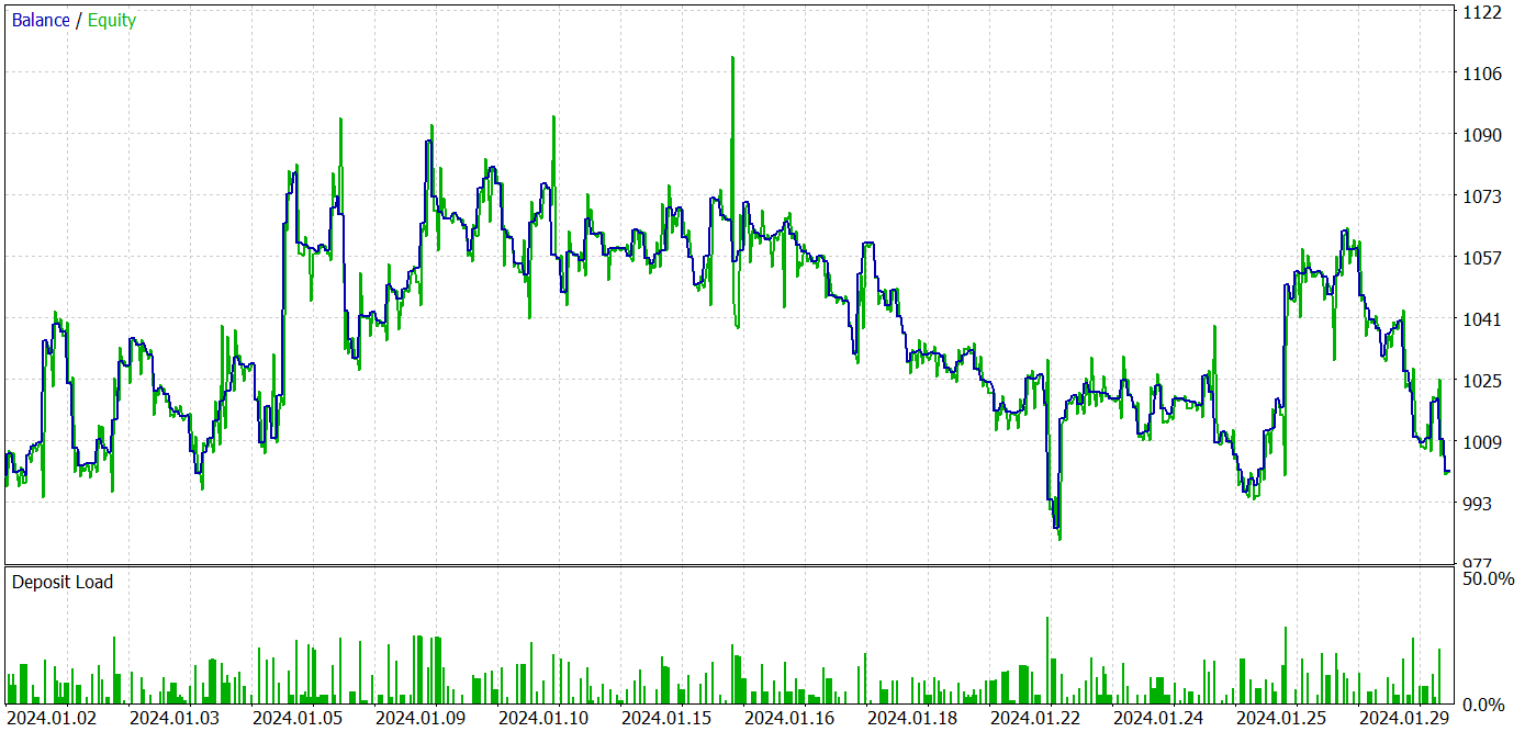
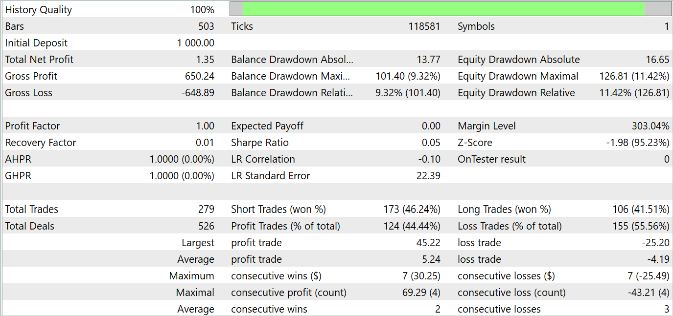
Based on the testing results, we see fluctuations in profitability on new data close to "0". Overall, we have maximum and average profits higher than similar loss indicators. However, the 44.4% winning trade rate did not allow for any profit to be made during the testing period.
Conclusion
In this article we got acquainted with a new method MLKV (Multi-Layer Key-Value), which is an innovative approach to more efficient memory use in Transformers. The main idea is to extend KV caching into multiple layers, which can significantly reduce memory usage.
In the practical part of the article, we implemented the proposed approaches using MQL5. We trained and tested models on real data. Our tests have shown that the proposed approaches can significantly reduce the costs of training and operating the model. However, this comes at the cost of the model's performance. As a conclusion, we should take a balanced approach to finding a compromise between costs and the model performance.
References
- MLKV: Multi-Layer Key-Value Heads for Memory Efficient Transformer Decoding
- Other articles from this series
Programs used in the article
| # | Name | Type | Description |
|---|---|---|---|
| 1 | Research.mq5 | EA | Example collection EA |
| 2 | ResearchRealORL.mq5 | EA | EA for collecting examples using the Real-ORL method |
| 3 | Study.mq5 | EA | Model training EA |
| 4 | StudyEncoder.mq5 | EA | Encoder training EA |
| 5 | Test.mq5 | EA | Model testing EA |
| 6 | Trajectory.mqh | Class library | System state description structure |
| 7 | NeuroNet.mqh | Class library | A library of classes for creating a neural network |
| 8 | NeuroNet.cl | Code Base | OpenCL program code library |
Translated from Russian by MetaQuotes Ltd.
Original article: https://www.mql5.com/ru/articles/15117
Warning: All rights to these materials are reserved by MetaQuotes Ltd. Copying or reprinting of these materials in whole or in part is prohibited.
This article was written by a user of the site and reflects their personal views. MetaQuotes Ltd is not responsible for the accuracy of the information presented, nor for any consequences resulting from the use of the solutions, strategies or recommendations described.

- Free trading apps
- Over 8,000 signals for copying
- Economic news for exploring financial markets
You agree to website policy and terms of use
And how do you realise that the network has learned something rather than generating random signals?
Actor's stochastic policy assumes some randomness of actions. However, in the process of learning, the range of scattering of random values is greatly narrowed. The point is that when organising a stochastic policy, 2 parameters are trained for each action: the mean value and the variance of the scatter of values. When training the policy, the mean value tends to the optimum and the variance tends to 0.
To understand how random the Agent's actions are I make several test runs for the same policy. If the Agent generates random actions, the result of all passes will be very different. For a trained policy the difference in results will be insignificant.
The Actor's stochastic policy assumes some randomness of actions. However, in the process of training, the range of random values scatter is strongly narrowed. The point is that when organising a stochastic policy, 2 parameters are trained for each action: the mean value and the variance of the scatter of values. When training the policy, the mean value tends to the optimum, and the variance tends to 0.
To understand how random the Agent's actions are I make several test runs for the same policy. If the Agent generates random actions, the result of all passes will be very different. For a trained policy the difference in results will be insignificant.
Got it, thanks.