
Neural Networks Made Easy (Part 92): Adaptive Forecasting in Frequency and Time Domains

Introduction
Time and frequency domain are two fundamental representations used to analyze time series data. In the time domain, analysis focuses on changes in amplitude over time, allowing the identification of local dependencies and transients within the signal. Conversely, frequency domain analysis aims to represent time series in terms of their frequency components, providing insight into the global dependencies and spectral characteristics of the data. Combining the advantages of both fields is a promising approach to address the problem of mixing different periodic patterns in real time series. The problem here is how to effectively combine the advantages of the time and frequency domains.
Compared with the achievements in the time domain, there are still many unexplored areas in the frequency domain. In recent articles we have seen some examples of using the frequency domain to better handle global time series dependencies. Direct forecasting in the frequency domain allows using more spectral information to improve the accuracy of time series forecasts. However, there are some problems associated with direct spectrum prediction in the frequency domain. One of these problems is the potential mismatch in frequency characteristics between the spectrum of known data being analyzed and the full spectrum of the time series being studied, which arises as a result of using the Discrete Fourier Transform (DFT). This mismatch makes it difficult to accurately represent information about specific frequencies across the entire spectrum of source data, leading to prediction inaccuracies.
Another problem is how to efficiently extract information about frequency combinations. Extracting spectral features is a challenging task because the harmonic series that occur in groups within the spectrum contain a significant amount of information.
The paper "ATFNet: Adaptive Time-Frequency Ensembled Network for Long-term Time Series Forecasting proposes the ATFNet method as a solution to the above mentioned problems. It includes time and frequency domain modules for simultaneous processing of local and global dependencies. In addition, the paper presents a new weighting mechanism that dynamically distributes weights between the two modules.
The authors of the method proposed an energy weighting of dominant harmonic series, which is capable of generating appropriate weights for modules in the time and frequency domains based on the level of periodicity demonstrated by the original data. This allows us to effectively exploit the advantages of both fields when working with time series with different periodic patterns.
In addition, the authors of the method introduce an extended DFT to align the spectrum of discrete frequencies of the original data and the full time series, which increases the accuracy of the representation of specific frequencies.
The authors of the method implement the attention mechanism in the frequency domain and propose complex spectral attention (CSA). This approach allows information to be collected from different combinations of frequency responses, providing an effective way to draw attention to frequency domain representations.
The article presents the results of experiments on eight real data sets, according to which ATFNet shows promising results and outperforms other state-of-the-art time series forecasting methods on many datasets.
1. ATFNet Algorithm
The authors of the ATFNet method employ a channel-independent scheme, which allows preventing the mixture of spectra from different channels. Since channels may possess different global patterns, mixing their spectra may have a negative impact on the performance of the model.
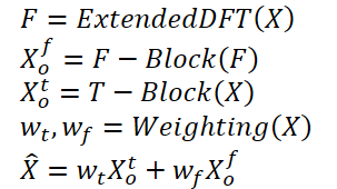
The T-block processes input univariate time series directly in the time domain. This results in an output of a certain predicted value of future values of the analyzed time series.
The authors of the method use the Extended Discrete Fourier Transform (DFT) to transform the original univariate time series data into the frequency domain, generating an extended frequency spectrum. The spectrum is then transformed back into the time domain using the inverse DFT (iDFT). As a result, F- block returns predicted values of the time series based on frequency characteristics.
Forecast results of the T-block and F-block are combined using adaptive weights to obtain the final result of the predicted values of the analyzed time series. These weights are determined based on the energy weighting of the Dominant Harmonic Series.
In general, the algorithm can be presented as follows:
The use of a traditional DFT may lead to a mismatch of frequencies between the spectra of the original data and the entire analyzed series. Therefore, forecasting models built on the analysis of a small block of initial data may not have access to complete and accurate information about the frequency characteristics of the entire analyzed time series. This results in less accurate forecasts when constructing the full time series.
To solve this problem, the authors of the method propose an Extended DFT, which overcomes the limitation imposed by the length of the analyzed source data. This allows us to obtain the original spectrum, which corresponds to the DFT frequency group of the complete series. Specifically, the authors of the ATFNet method replace the original complex exponential basis with the DFT basis of the complete full series:
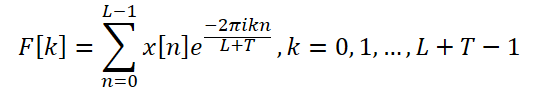
Thus, we obtain a spectrum of frequency characteristics of length L + T, which aligns with the DFT spectrum of the complete analyzed series (initial + forecast data). For real time series, the conjugate symmetry of the output spectrum is an important property of DFT. Using this property, we can reduce computational costs by considering only the first half of the frequency spectrum of the original data, since the second half provides redundant information.
The architecture of F-Block is based on the Transformer Encoder, all parameters of which have complex values. All computations in the F-block are performed in the field of complex numbers.
In addition, the authors of the method use RevIN to process the original spectrum of frequency characteristics F. Although RevIN is originally developed to eliminate distribution shifts in the time domain, the authors of the method found it to be effective in processing spectra in the frequency domain as well. This approach allows transforming spectra of series with different global characteristics into a comparable distribution. Before analysis, frequency characteristics F are normalized. After processing the data, we add the statistical characteristics of the frequency distribution back.
Since there are few chronological dependencies in the frequency domain spectrum, the authors of the method do not use positional encoding in the F-block.
Additionally, the authors of the method used a modified multi-head attention mechanism. For each head h = 1, 2, ..., H, the built-in spectrum Fd is projected on spectrum measurement using trained projections. After that, a complex scalar product of attention is performed on each head.
ATFNet also uses LayerNorm and FeedForward layers with residual connections similarly to Transformer, which are extended to the field of complex numbers.
After M Encoder layers, the results of the attention block work are linearly projected onto the horizon of the full series. The obtained frequency characteristics are projected into the time domain using iDFT. The last T points (part of the forecast) are accepted as the final result of the F-Block.
It should be noted that the F-Block uses the full architecture of a complex value neural network (CVNN).
The T-Block is responsible for capturing local dependencies in time series, which are easier to process in the time domain. In this block, the authors use the time series segmentation method that is already familiar to us. PatchTST is an intuitive and efficient way to capture local dependencies in time series. It also uses RevIN to solve the problem of distribution bias.
Periodic time series consistently exhibit the existence of at least one harmonic group in their frequency domain spectrum, with the dominant harmonic group exhibiting the highest concentration of spectral energy. Conversely, this characteristic is rarely observed in the spectrum of non-periodic time series, where the energy distribution is more uniform. The authors of the ATFNet method show that the degree of energy concentration within the dominant harmonic series in the frequency spectrum can reflect the periodicity of the time series. The ratio of the energy of the dominant harmonic series to the total energy of the spectrum can serve as a metric for quantitatively assessing the concentration of energy. Intuitively, when a time series exhibits a more pronounced periodic structure, it can be decomposed into components. Therefore, such a time series has a higher concentration of energy within the dominant harmonic series.
Based on this property, ATFNet authors use the energy fraction of the dominant harmonic series as an indicator for quantitatively assessing the degree of periodicity of the time series. To identify the dominant harmonic series, the most important task is to determine the fundamental frequency. There are different approaches that can be used here:
- A naive method that identifies the frequency with the highest amplitude value as the fundamental frequency.
- Rule-based pitch detection algorithms.
- Data-driven pitch detection algorithms.
The ATFNet algorithm allows us to use any approach to determining the fundamental frequency. The authors of the method consider this component together with its harmonics and calculate the total energy Eh. Then the weights of the F-Block are determined by calculating the ratio of the energy of the dominant frequency to the total energy of the spectrum.
In the paper, the authors of the method conducted a series of experiments to evaluate the effectiveness of various methods for determining the dominant frequency. They concluded that the naive method is the leader in terms of the ratio of the accuracy of the results to the cost of computations. It demonstrates commendable accuracy across a majority of real-world time series datasets while maintaining low computational cost.
Conversely, alternative approaches are hampered by the problem of computational complexity. In addition, data-driven methods require labeled step data, which is often difficult to obtain, which poses a serious obstacle to their practical use. Therefore, in their experiments, the authors of the ATFNet method use a naive method by default to detect the fundamental frequency.
The original visualization of the AFTNet method is presented below.
2. Implementing basic operations with complex numbers
In previous articles, we have already discussed a little complex numbers. They are convenient to use to describe the spectrum of frequency characteristics. We use the real part to represent the signal amplitude and the imaginary part to represent the phase shift. However, having received from DFT a signal in complex form, we worked separately with the real and imaginary parts. Then, using iDFT, we transformed the frequency characteristics obtained in this way into the time domain.
Despite the simplicity of implementing the approach to analyzing the real and imaginary parts as separate entities, this approach is not optimal. ATFNet authors examine in detail both approaches to processing complex numbers and come to the conclusion that the analysis of the real and imaginary parts as separate entities leads to a loss of information. Therefore, to implement the proposed method, we need to modify the attention block to work with complex numbers.
Unfortunately, OpenCL does not support complex numbers. Therefore, we have to implement the basic operations of complex algebra ourselves.
As already mentioned above, a complex number consists of a real part and an imaginary part:
![]()
where a is the real part,
b is the imaginary part,
i is the imaginary unit.
To save the complex number on the OpenCL side, it is convenient to use a vector of 2 elements float2.
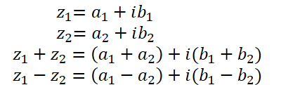
Addition and subtraction of complex numbers almost completely repeat those implemented in OpenCL vector operations. Therefore, we will not discuss them now.
But multiplication of complex numbers is a little more complicated.
![]()
To implement this operation, we will create the ComplexMul function in the OpenCL program.
float2 ComplexMul(const float2 a, const float2 b)
  {
   float2 result = 0;
   result.x = a.x * b.x - a.y * b.y;
   result.y = a.x * b.y + a.y * b.x;
   return result;
  }
The function takes two float2 vectors as parameters and returns the result in the same format. In this way we create something very similar to correct operations with complex variables.
The division of complex numbers has a more complex form:
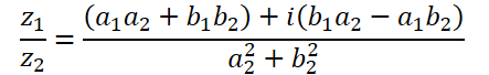
To perform this operation, let's create the ComplexDiv function.
float2 ComplexDiv(const float2 a, const float2 b)
  {
   float2 result = 0;
   float z = pow(b.x, 2) + pow(b.y, 2);
   if(z > 0)
     {
      result.x = (a.x * b.x + a.y * b.y) / z;
      result.y = (a.y * b.x - a.x * b.y) / z;
     }
   return result;
  }
The absolute value of a complex number is a real number that indicates the energy of the frequency component:
![]()
Let's implement this in the ComplexAbs function.
float ComplexAbs(float2 a)
  {
   return sqrt(pow(a.x, 2) + pow(a.y, 2));
  }
The formula for extracting the square root of a complex number is a little more complicated:
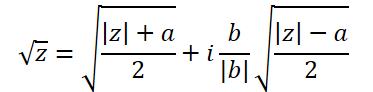
To implement it, let's create another function, ComplexSqrt.
float2 ComplexSqrt(float2 a)
  {
   float2 result = 0;
   float z = ComplexAbs(a);
   result.x = sqrt((z + a.x) / 2);
   result.y = sqrt((z - a.x) / 2);
   if(a.y < 0)
      result.y *= (-1);
//---
   return result;
  }
When implementing the Self-Attention algorithm, we normalize the dependence coefficients using the SoftMax function. To implement it in the domain of complex numbers, we will need the exponent of the complex number:
![]()
In the code, we implement the function as follows:
float2 ComplexExp(float2 a)
  {
   float2 result = exp(clamp(a.x, -20.0f, 20.0f));
   result.x *= cos(a.y);
   result.y *= sin(a.y);
   return result;
  }
3. Complex Attention Layer
We have carried out the preparatory work and implemented basic mathematical operations with complex numbers. Now we move on to the next step, where we will create a attention neural layer class using complex number mathematics: CNeuronComplexMLMHAttention.
We create the new class based on a similar attention layer for real values CNeuronMLMHAttentionOCL. The advantage of this approach is that we can make maximum reuse of the already existing and pre-configured top-level functionality. So, we only need to redefine methods at the lower level to be able to work with complex values. The structure of the new class is shown below.
class CNeuronComplexMLMHAttention :  public CNeuronMLMHAttentionOCL
  {
protected:
   virtual bool      ConvolutionForward(CBufferFloat *weights, CBufferFloat *inputs, CBufferFloat *outputs,

                                        uint window, uint window_out, ENUM_ACTIVATION activ, uint step = 0);
   virtual bool      AttentionScore(CBufferFloat *qkv, CBufferFloat *scores, bool mask = false);
   virtual bool      AttentionOut(CBufferFloat *qkv, CBufferFloat *scores, CBufferFloat *out);
   virtual bool      ConvolutuionUpdateWeights(CBufferFloat *weights, CBufferFloat *gradient, CBufferFloat *inputs,
                                               CBufferFloat *momentum1, CBufferFloat *momentum2,
                                               uint window, uint window_out, uint step = 0);
   virtual bool      ConvolutionInputGradients(CBufferFloat *weights, CBufferFloat *gradient, CBufferFloat *inputs,
                                               CBufferFloat *inp_gradient, uint window, uint window_out,
                                               uint activ, uint shift_out = 0, uint step = 0);
   virtual bool      AttentionInsideGradients(CBufferFloat *qkv, CBufferFloat *qkv_g, CBufferFloat *scores,
                                              CBufferFloat *gradient);
   virtual bool      SumAndNormilize(CBufferFloat *tensor1, CBufferFloat *tensor2, CBufferFloat *out,
                                     int dimension, bool normilize = true, int shift_in1 = 0, int shift_in2 = 0,
                                     int shift_out = 0, float multiplyer = 0.5f);

public:
                     CNeuronComplexMLMHAttention(void) {};
                    ~CNeuronComplexMLMHAttention(void) {};
   virtual bool      Init(uint numOutputs, uint myIndex, COpenCLMy *open_cl, uint window, uint window_key, uint heads,
                          uint units_count, uint layers, ENUM_OPTIMIZATION optimization_type, uint batch);
   //---
   virtual int       Type(void)   const   {  return defNeuronComplexMLMHAttentionOCL;   }
  };
The notable thing about the structure of the new class is that it does not declare a single internal object or variable. In the process of implementing the functionality, we will use inherited objects and variables.
Furthermore, the class structure only declares the overriding of methods in the protected block. All the methods were previously declared in the parent class. However, there are no high-level feed-forward and backpropagation methods (feedForward, calcInputGradients and updateInputWeights), in which we usually build the class algorithm. This is because we completely preserve the sequence of actions of the parent class algorithm. However, to work with complex values, we need to double the size of the data buffers, because the imaginary part of the complex value is added to each real value. In addition, we need to implement complex number mathematics into the algorithm. As you know, we perform almost all mathematical operations on the OpenCL side. Therefore, in addition to redefining the lower-level methods, we will also have to make changes to the OpenCL program kernels.
3.1 Class initialization method
The work of each class begins with its initialization. As mentioned above, we do not declare any nested objects or variables in our new class. That is why the constructor and the destructor are empty. Initialization of inherited objects is performed in the Init method. As usual, in the parameters of this method, we receive from the caller the main constants that define the architecture of the class. As you can see, the structure of the method parameters is the same as in the similar method of the parent class. This is not surprising. Because we completely preserve the basic attention algorithm and the structure of the parent class. However, we will completely rewrite the method itself.
bool CNeuronComplexMLMHAttention::Init(uint numOutputs, uint myIndex, COpenCLMy *open_cl,
                                       uint window, uint window_key, uint heads, uint units_count, uint layers,
                                       ENUM_OPTIMIZATION optimization_type, uint batch)
  {
   if(!CNeuronBaseOCL::Init(numOutputs, myIndex, open_cl, 2 * window * units_count, optimization_type, batch))
      return false;
In the method body, as usual, we call the initialization method of the parent class. Please pay attention to the following two points:
- We call the initialization method not of the direct parent CNeuronMLMHAttentionOCL, but of the base neural layer base class CNeuronBaseOCL. The reason is that the initialization of nested objects of the CNeuronMLMHAttentionOCL class is not needed since we have to redefine all buffers with increased sizes to be able to store complex numbers.
- When calling the parent class method, we increase the layer size by 2 times. This is because we expect the layer operation result in complex values.
Make sure to check the logical result of the operations of the parent class method.
After successfully initializing the objects inherited from the base class of the neural layer, we save the main parameters of the architecture of the created layer.
   iWindow = window;
   iWindowKey = fmax(window_key, 1);
   iUnits = units_count;
   iHeads = fmax(heads, 1);
   iLayers = fmax(layers, 1);
In the next step, we calculate the sizes of all buffers we are creating. We need to store complex values. Therefore, all buffers are increased by 2 times compared to the parent class.
   uint num = 2 * 3 * iWindowKey * iHeads * iUnits;     //Size of QKV tensor
   uint qkv_weights = 2 * 3 * (iWindow + 1) * iWindowKey * iHeads; //Size of weights' matrix of QKV tenzor
   uint scores = 2 * iUnits * iUnits * iHeads;          //Size of Score tensor
   uint mh_out = 2 * iWindowKey * iHeads * iUnits;      //Size of multi-heads self-attention
   uint out = 2 * iWindow * iUnits;                     //Size of our tensore
   uint w0 = 2 * (iWindowKey + 1) * iHeads * iWindow;   //Size W0 tensor
   uint ff_1 = 2 * 4 * (iWindow + 1) * iWindow;         //Size of weights' matrix 1-st feed forward layer
   uint ff_2 = 2 * (4 * iWindow + 1) * iWindow;         //Size of weights' matrix 2-nd feed forward layer
Then we organize a loop according to the number of created nested attention layers. In its body, we initialize the nested objects.
   for(uint i = 0; i < iLayers; i++)
     {
      CBufferFloat *temp = NULL;
Here we first create a nested loop of 2 iterations in which we initialize objects to record the feed-forward pass data and the corresponding error gradients.
      for(int d = 0; d < 2; d++)
        {
         //--- Initilize QKV tensor
         temp = new CBufferFloat();
         if(CheckPointer(temp) == POINTER_INVALID)
            return false;
         if(!temp.BufferInit(num, 0))
            return false;
         if(!temp.BufferCreate(OpenCL))
            return false;
         if(!QKV_Tensors.Add(temp))
            return false;
First we create a concatenated buffer of Query, Key and Value entities. Next, according to the Self-Attention algorithm, we need a buffer to write the matrix of dependence coefficients.
         //--- Initialize scores
         temp = new CBufferFloat();
         if(CheckPointer(temp) == POINTER_INVALID)
            return false;
         if(!temp.BufferInit(scores, 0))
            return false;
         if(!temp.BufferCreate(OpenCL))
            return false;
         if(!S_Tensors.Add(temp))
            return false;
The following buffer will store the results of multi-headed attention:
         //--- Initialize multi-heads attention out
         temp = new CBufferFloat();
         if(CheckPointer(temp) == POINTER_INVALID)
            return false;
         if(!temp.BufferInit(mh_out, 0))
            return false;
         if(!temp.BufferCreate(OpenCL))
            return false;
         if(!AO_Tensors.Add(temp))
            return false;
We will then reduce the size down to the input level.
         //--- Initialize attention out
         temp = new CBufferFloat();
         if(CheckPointer(temp) == POINTER_INVALID)
            return false;
         if(!temp.BufferInit(out, 0))
            return false;
         if(!temp.BufferCreate(OpenCL))
            return false;
         if(!FF_Tensors.Add(temp))
            return false;
The Attention block is followed by the FeedForward block consisting of 2 fully connected layers:
         //--- Initialize Feed Forward 1
         temp = new CBufferFloat();
         if(CheckPointer(temp) == POINTER_INVALID)
            return false;
         if(!temp.BufferInit(4 * out, 0))
            return false;
         if(!temp.BufferCreate(OpenCL))
            return false;
         if(!FF_Tensors.Add(temp))
            return false;
         //--- Initialize Feed Forward 2
         if(i == iLayers - 1)
           {
            if(!FF_Tensors.Add(d == 0 ? Output : Gradient))
               return false;
            continue;
           }
         temp = new CBufferFloat();
         if(CheckPointer(temp) == POINTER_INVALID)
            return false;
         if(!temp.BufferInit(out, 0))
            return false;
         if(!temp.BufferCreate(OpenCL))
            return false;
         if(!FF_Tensors.Add(temp))
            return false;
        }
We have initialized buffers to store the feed-forward pass results and the corresponding error gradients. However, to perform the operations, we need learnable weight parameters. First, we fill in the matrix of learnable parameters for generating the Query, Key and Value entities:
      //--- Initilize QKV weights
      temp = new CBufferFloat();
      if(CheckPointer(temp) == POINTER_INVALID)
         return false;
      if(!temp.Reserve(qkv_weights))
         return false;
      float k = (float)(1 / sqrt(iWindow + 1));
      for(uint w = 0; w < qkv_weights; w++)
        {
         if(!temp.Add(GenerateWeight() * 2 * k - k))
            return false;
        }
      if(!temp.BufferCreate(OpenCL))
         return false;
      if(!QKV_Weights.Add(temp))
         return false;
Then we generate the parameters of the multi-headed attention dimensionality reduction layer:
      //--- Initilize Weights0
      temp = new CBufferFloat();
      if(CheckPointer(temp) == POINTER_INVALID)
         return false;
      if(!temp.Reserve(w0))
         return false;
      for(uint w = 0; w < w0; w++)
        {
         if(!temp.Add(GenerateWeight() * 2 * k - k))
            return false;
        }
      if(!temp.BufferCreate(OpenCL))
         return false;
      if(!FF_Weights.Add(temp))
         return false;
Let's add FeedForward block parameters:
      //--- Initilize FF Weights
      temp = new CBufferFloat();
      if(CheckPointer(temp) == POINTER_INVALID)
         return false;
      if(!temp.Reserve(ff_1))
         return false;
      for(uint w = 0; w < ff_1; w++)
        {
         if(!temp.Add(GenerateWeight() * 2 * k - k))
            return false;
        }
      if(!temp.BufferCreate(OpenCL))
         return false;
      if(!FF_Weights.Add(temp))
         return false;
      //---
      temp = new CBufferFloat();
      if(CheckPointer(temp) == POINTER_INVALID)
         return false;
      if(!temp.Reserve(ff_2))
         return false;
      k = (float)(1 / sqrt(4 * iWindow + 1));
      for(uint w = 0; w < ff_2; w++)
        {
         if(!temp.Add(GenerateWeight() * 2 * k - k))
            return false;
        }
      if(!temp.BufferCreate(OpenCL))
         return false;
      if(!FF_Weights.Add(temp))
         return false;
During the model parameter training process, we will need buffers to record the training moments. The number of such buffers depends on the parameter learning method used.
      for(int d = 0; d < (optimization == SGD ? 1 : 2); d++)
        {
         temp = new CBufferFloat();
         if(CheckPointer(temp) == POINTER_INVALID)
            return false;
         if(!temp.BufferInit(qkv_weights, 0))
            return false;
         if(!temp.BufferCreate(OpenCL))
            return false;
         if(!QKV_Weights.Add(temp))
            return false;
         temp = new CBufferFloat();
         if(CheckPointer(temp) == POINTER_INVALID)
            return false;
         if(!temp.BufferInit(w0, 0))
            return false;
         if(!temp.BufferCreate(OpenCL))
            return false;
         if(!FF_Weights.Add(temp))
            return false;
         //--- Initilize FF Weights
         temp = new CBufferFloat();
         if(CheckPointer(temp) == POINTER_INVALID)
            return false;
         if(!temp.BufferInit(ff_1, 0))
            return false;
         if(!temp.BufferCreate(OpenCL))
            return false;
         if(!FF_Weights.Add(temp))
            return false;
         temp = new CBufferFloat();
         if(CheckPointer(temp) == POINTER_INVALID)
            return false;
         if(!temp.BufferInit(ff_2, 0))
            return false;
         if(!temp.BufferCreate(OpenCL))
            return false;
         if(!FF_Weights.Add(temp))
            return false;
        }
     }
//---
   return true;
  }
Make sure to check the result of each iteration of this method, since during the training and operation of the model, the absence of even one of the necessary buffers will lead to a critical error.
After initializing all nested objects, we terminate the method and return the logical value of the performed operations to the caller.
3.2 Feed-forward pass
After initializing the class, we proceed to organizing the feed-forward pass. Even though we inherit the high-level algorithm from the parent class, we still have some work to do with the feed-forward methods at the low level. We will arrange operations in the sequence of the Self-Attention algorithm.
The input data of the layer is first transformed into Query, Key and Value entities. To generate them in the parent class, we used the forward pass kernel of the convolutional layer. In this implementation, we will follow the same approach. Additionally, to work with complex variables, we need to create a new kernel called FeedForwardComplexConv on the OpenCL program side.
In the kernel parameters, we pass pointers to 3 data buffers: the matrix of training parameters, the input data, and a buffer for writing the results.
__kernel void FeedForwardComplexConv(__global float2 *matrix_w,
                                     __global float2 *matrix_i,
                                     __global float2 *matrix_o,
                                     int inputs,
                                     int step,
                                     int window_in,
                                     int activation
                                    )
  {
   size_t i = get_global_id(0);
   size_t out = get_global_id(1);
   size_t w_out = get_global_size(1);
Note that on the main program side, we still use data buffers of type float but of increased size. In the kernel on the OpenCL program side, we specify type float2 for data buffers. This is exactly the type of data we used above when creating functions of complex variables.
In the method body, we identify the current thread in the two-dimensional task space. The first dimension indicates the element in the result sequence, and the second dimension indicates the filter used. In our case, it will indicate the position in the concatenated vector of entities describing one element of the sequence being analyzed.
Based on the data obtained, we determine the offset in the data buffers:
   int w_in = window_in;
   int shift_out = w_out * i;
   int shift_in = step * i;
   int shift = (w_in + 1) * out;
   int stop = (w_in <= (inputs - shift_in) ? w_in : (inputs - shift_in));
Next we create a loop to compute the product of vectors:
   float2 sum = matrix_w[shift + w_in];
   for(int k = 0; k <= stop; k ++)
      sum += ComplexMul(matrix_i[shift_in + k], matrix_w[shift + k]);
Note that to compute the product of 2 complex quantities we use the ComplexMul function created above. We use basic vector operations to sum values.
In addition, since we have declared float2 vector type for data buffers, we can access them as normal floating-point data buffers without offset adjustment. At each operation, two elements are extracted from the buffer: the real and imaginary parts of the complex number.
Next we check the computed value. In case of variable overflow, we change its value to 0:
   if(isnan(sum.x) || isnan(sum.y) || isinf(sum.x) || isinf(sum.y))
      sum = (float2)0;
Now we just need to calculate the activation function and save the value to the result buffer.
   switch(activation)
     {
      case 0:
         sum = ComplexTanh(sum);
         break;
      case 1:
         sum = ComplexDiv((float2)(1, 0), (float2)(1, 0) + ComplexExp(-sum));
         break;
      case 2:
         if(sum.x < 0)
            sum.x *= 0.01f;
         if(sum.y < 0)
            sum.y *= 0.01f;
         break;
      default:
         break;
     }
   matrix_o[out + shift_out] = sum;
  }
To call the above created kernel on the main program side, we will override the CNeuronComplexMLMHAttention::ConvolutionForward method. Notice that we are overriding the method rather than creating a new one. Therefore, it is very important to preserve the full parameter structure of the similar method of the parent class. Only overriding the method will allow us to call this method from the top-level feed-forward pass method of the parent class without making any adjustments to it.
bool CNeuronComplexMLMHAttention::ConvolutionForward(CBufferFloat *weights, CBufferFloat *inputs,
                                                     CBufferFloat *outputs, uint window, uint window_out,
                                                     ENUM_ACTIVATION activ, uint step = 0)
  {
   if(CheckPointer(OpenCL) == POINTER_INVALID || CheckPointer(weights) == POINTER_INVALID ||
      CheckPointer(inputs) == POINTER_INVALID || CheckPointer(outputs) == POINTER_INVALID)
      return false;
In the body of the method, we first check the relevance of the received pointers to objects. And then we check if there are data buffers on the OpenCL context side.
   if(weights.GetIndex() < 0)
      return false;
   if(inputs.GetIndex() < 0)
      return false;
   if(outputs.GetIndex() < 0)
      return false;
   if(step == 0)
      step = window;
After successfully passing the control block, we define the task space for the kernel and the offset in it:
   uint global_work_offset[2] = {0, 0};
   uint global_work_size[2];
   global_work_size[0] = outputs.Total() / (2 * window_out);
   global_work_size[1] = window_out;
Then we pass all the necessary parameters to the kernel, while controlling the execution of operations:
   if(!OpenCL.SetArgumentBuffer(def_k_FeedForwardComplexConv, def_k_ffc_matrix_w, weights.GetIndex()))
     {
      printf("Error of set parameter kernel %s: %d; line %d", __FUNCTION__, GetLastError(), __LINE__);
      return false;
     }
   if(!OpenCL.SetArgumentBuffer(def_k_FeedForwardComplexConv, def_k_ffc_matrix_i, inputs.GetIndex()))
     {
      printf("Error of set parameter kernel %s: %d; line %d", __FUNCTION__, GetLastError(), __LINE__);
      return false;
     }
   if(!OpenCL.SetArgumentBuffer(def_k_FeedForwardComplexConv, def_k_ffc_matrix_o, outputs.GetIndex()))
     {
      printf("Error of set parameter kernel %s: %d; line %d", __FUNCTION__, GetLastError(), __LINE__);
      return false;
     }
   if(!OpenCL.SetArgument(def_k_FeedForwardComplexConv, def_k_ffc_inputs, (int)(inputs.Total() / 2)))
     {
      printf("Error of set parameter kernel %s: %d; line %d", __FUNCTION__, GetLastError(), __LINE__);
      return false;
     }
   if(!OpenCL.SetArgument(def_k_FeedForwardComplexConv, def_k_ffc_step, (int)step))
     {
      printf("Error of set parameter kernel %s: %d; line %d", __FUNCTION__, GetLastError(), __LINE__);
      return false;
     }
   if(!OpenCL.SetArgument(def_k_FeedForwardComplexConv, def_k_ffc_window_in, (int)window))
     {
      printf("Error of set parameter kernel %s: %d; line %d", __FUNCTION__, GetLastError(), __LINE__);
      return false;
     }
   if(!OpenCL.SetArgument(def_k_FeedForwardComplexConv, def_k_ffс_window_out, (int)window_out))
     {
      printf("Error of set parameter kernel %s: %d; line %d", __FUNCTION__, GetLastError(), __LINE__);
      return false;
     }
   if(!OpenCL.SetArgument(def_k_FeedForwardComplexConv, def_k_ffc_activation - 1, (int)activ))
     {
      printf("Error of set parameter kernel %s: %d; line %d", __FUNCTION__, GetLastError(), __LINE__);
      return false;
     }
After that, we place the kernel in the execution queue and complete the method:
   if(!OpenCL.Execute(def_k_FeedForwardComplexConv, 2, global_work_offset, global_work_size))
     {
      string error;
      CLGetInfoString(OpenCL.GetContext(), CL_ERROR_DESCRIPTION, error);
      printf("Error of execution kernel %s: %s", __FUNCSIG__, error);
      return false;
     }
//---
   return true;
  }
The algorithm for placing kernels in the execution queue is quite uniform. There may be differences in the size of the task space and variations with variables. In order to save your time and reduce the volume of the article, we will not dwell further on the of kernel queuing methods. Their full code can be found in the attachment. Let's dwell in detail the algorithms for constructing these kernels.
We continue following the Self-Attention algorithm. After defining the Query, Key and Value entities, we move on to defining the dependence coefficients. To define the, we need to multiply the Query matrix by the transposed Key matrix. The result matrix is normalized using the SoftMax function.
The described functionality is executed in the ComplexMHAttentionScore kernel, which will be called from the CNeuronComplexMLMHAttention::AttentionScore method.
__kernel void ComplexMHAttentionScore(__global float2 *qkv,
                                      __global float2 *score,
                                      int dimension,
                                      int mask
                                     )
  {
   int q = get_global_id(0);
   int h = get_global_id(1);
   int units = get_global_size(0);
   int heads = get_global_size(1);
In the parameters, the kernel receives pointers to 2 data buffers. Concatenated buffer of entities as input. And a buffer for writing the results.
The specified kernel is run in a two-dimensional task space. The first dimension defines a row of the Query matrix, and the second one defines an active attention head. Thus, each separate instance of the running kernel performs operations to calculate 1 row of the matrix of dependence coefficients within 1 attention head.
In the kernel body, we identify the current thread in both dimensions of the task space and determine the offsets into the data buffers:
   int shift_q = dimension * (h + 3 * q * heads);
   int shift_s = units * (h + q * heads);
Then we define the data normalization factor:
   float2 koef = (float2)(sqrt((float)dimension), 0);
   if(koef.x < 1)
      koef.x = 1;
Create a loop to compute the dependence coefficients:
   float2 sum = 0;
   for(int k = 0; k < units; k++)
     {
      if(mask > 0 && k > q)
        {
         score[shift_s + k] = (float2)0;
         continue;
        }
It should be noted here that the presented algorithm implements data masking, which allows limiting the so-called "look-ahead". The model only analyzes the coefficients of dependence to previous tokens. For subsequent tokens, the dependency coefficients are set to 0 so that the model cannot receive information "from the future" during the training process. This functionality is enabled using the mask flag, which is passed in the kernel parameters.
Next, in a nested loop, we calculate the next element of the dependency vector by multiplying 2 vectors.
      float2 result = (float2)0;
      int shift_k = dimension * (h + heads * (3 * k + 1));
      for(int i = 0; i < dimension; i++)
         result += ComplexMul(qkv[shift_q + i], qkv[shift_k + i]);
We calculate the exponent for the result of the product:
result = ComplexExp(ComplexDiv(result, koef));
It is necessary to define variable overflow:
      if(isnan(result.x) || isnan(result.y) || isinf(result.x) || isinf(result.y))
         result = (float2)0;
We write the result to the results buffer and add it to the total sum for subsequent normalization.
      score[shift_s + k] = result;
      sum += result;
     }
At the end of the kernel, we normalize the calculated row of the matrix of dependence coefficients:
   if(ComplexAbs(sum) > 0)
      for(int k = 0; k < units; k++)
         score[shift_s + k] = ComplexDiv(score[shift_s + k], sum);
  }
The Score matrix of dependence coefficients obtained in this way is used to calculate the results of the attention block. Here we need to multiply the obtained matrix of coefficients by the matrix of Value entities. This work is done in the ComplexMHAttentionOut kernel. Similar to the previous one, this kernel works in the same 2-dimensional task space.
__kernel void ComplexMHAttentionOut(__global float2 *scores,
                                    __global float2 *qkv,
                                    __global float2 *out,
                                    int dimension
                                   )
  {
   int u = get_global_id(0);
   int units = get_global_size(0);
   int h = get_global_id(1);
   int heads = get_global_size(1);
In the kernel body, we identify the current thread in the task space and determine the offsets into the data buffers:
   int shift_s = units * (h + heads * u);
   int shift_out = dimension * (h + heads * u);
After that, we create a system of nested loops to perform mathematical operations for multiplying the Valuematrix by the corresponding line of dependence coefficients:
   for(int d = 0; d < dimension; d++)
     {
      float2 result = (float2)0;
      for(int v = 0; v < units; v++)
        {
         int shift_v = dimension * (h + heads * (3 * v + 2)) + d;
         result += ComplexMul(scores[shift_s + v], qkv[shift_v]);
        }
      out[shift_out + d] = result;
     }
  }
The result of multi-headed attention is then consolidated into a single tensor and reduced in dimension to the size of the input data tensor. Then we perform the operations of the FeedForward block. These operations are performed using the FeedForwardComplexConv kernel described above. This concludes our description of the kernel algorithms for performing feed-forward pass operations. You can see the full code of all kernels, as well as the methods that call them, in the attachment.
3.3 Implementing the Backpropagation pass
The feed-forward pass functionality is ready. Next, we proceed to implement the backpropagation algorithms. This work is similar to that performed above for the feed-forward pass. We exploit the high-level algorithms inherited from the parent class and override the low-level methods.
As mentioned above, we will not consider the algorithms of the methods that place kernels in the execution queue. They are all the same. Let's pay more attention to the analysis of kernel algorithms on the OpenCL program side.
The most used in the feed-forward pass was the FeedForwardComplexConv kernel. This is a universal block that we use at different stages. Naturally, we begin the construction of backpropagation algorithms precisely with the kernel for propagating the error gradient through the specified block. We implement this functionality in the CalcHiddenGradientComplexConv kernel.
__kernel void CalcHiddenGradientComplexConv(__global float2 *matrix_w,
                                            __global float2 *matrix_g,
                                            __global float2 *matrix_o,
                                            __global float2 *matrix_ig,
                                            int outputs,
                                            int step,
                                            int window_in,
                                            int window_out,
                                            int activation,
                                            int shift_out
                                           )
  {
   size_t i = get_global_id(0);
   size_t inputs = get_global_size(0);
The kernel runs in a one-dimensional task space according to the number of elements in the input data buffer. Each individual thread of a given kernel collects error gradients from all elements that are affected by the analyzed input element.
In the kernel body, we identify the current thread and determine the offsets into the data buffers. We also declare the necessary local variables:
   float2 sum = (float2)0;
   float2 out = matrix_o[shift_out + i];
   int start = i - window_in + step;
   start = max((start - start % step) / step, 0);
   int stop = (i + step - 1) / step;
   if(stop > (outputs / window_out))
      stop = outputs / window_out;
After that, we create a system of loops. In their body, we will collect the total error gradient, taking into account the influence of the analyzed element on the overall result:
   for(int h = 0; h < window_out; h ++)
     {
      for(int k = start; k < stop; k++)
        {
         int shift_g = k * window_out + h;
         int shift_w = (stop - k - 1) * step + i % step + h * (window_in + 1);
         if(shift_g >= outputs || shift_w >= (window_in + 1) * window_out)
            break;
         sum += ComplexMul(matrix_g[shift_out + shift_g], matrix_w[shift_w]);
        }
     }
After exiting the loop, we check for variable overflow:
   if(isnan(sum.x) || isnan(sum.y) || isinf(sum.x) || isinf(sum.y))
      sum = (float2)0;
We also adjust the obtained error gradient by the derivative of the activation function:
   switch(activation)
     {
      case 0:
         sum = ComplexMul(sum, (float2)1.0f - ComplexMul(out, out));
         break;
      case 1:
         sum = ComplexMul(sum, ComplexMul(out, (float2)1.0f - out));
         break;
      case 2:
         if(out.x < 0.0f)
            sum.x *= 0.01f;
         if(out.y < 0.0f)
            sum.y *= 0.01f;
         break;
      default:
         break;
     }
   matrix_ig[i] = sum;
  }
We will save the final result in the error gradient buffer of the previous layer.
Next, let's consider the kernel for propagating the error gradient through the attention block ComplexMHAttentionGradients. This kernel presents a rather complex algorithm, which can be conditionally divided into 3 blocks according to the number of entities for which the error gradient value is determined.
__kernel void ComplexMHAttentionGradients(__global float2 *qkv, __global float2 *qkv_g,
                                          __global float2 *scores, __global float2 *gradient)
  {
   size_t u = get_global_id(0);
   size_t h = get_global_id(1);
   size_t d = get_global_id(2);
   size_t units = get_global_size(0);
   size_t heads = get_global_size(1);
   size_t dimension = get_global_size(2);
There are quite a lot of operations performed in this kernel. In order to reduce the overall execution time, during the model training process, we tried to parallelize the operations related to the computation of values for individual variables. To make thread identification transparent and intuitive, we created a 3-dimensional task space for this kernel. As in the attention block feed-forward pass methods, here we use the sequence element and the attention head. The third dimension of the task space is used for the position of the element in the tensor describing the sequence element. Thus, despite the large number of operations, each individual thread will write only 3 values to the result buffer. In this case, it is a concatenated buffer of error gradients for the Query, Key and Value entities.
In the kernel body, we first identify the thread in the task space and determine the offsets into the data buffers:
   float2 koef = (float2)(sqrt((float)dimension), 0);
   if(koef.x < 1)
      koef.x = 1;
//--- init
   const int shift_q = dimension * (heads * 3 * u + h);
   const int shift_k = dimension * (heads * (3 * u + 1) + h);
   const int shift_v = dimension * (heads * (3 * u + 2) + h);
   const int shift_g = dimension * (heads * u + h);
   int shift_score = h * units;
   int step_score = units * heads;
Then we determine the error gradient for the analyzed element of the Value matrix. We multiply a separate column of the error gradient tensor at the output of the attention block by the corresponding column of the dependence coefficient matrix:
//--- Calculating Value's gradients
   float2 sum = (float2)0;
   for(int i = 0; i < units; i++)
      sum += ComplexMul(gradient[(h + i * heads) * dimension + d], scores[shift_score + u + i * step_score]);
   qkv_g[shift_v + d] = sum;
In the next step, we determine the error gradient for the analyzed element of the Query entity. This entity does not have a direct influence on the result. There is only an indirect influence through the matrix of dependence coefficients. Therefore, we first need to find the error gradient for the corresponding row of the matrix of dependence coefficients. Data normalization using the SoftMax function complicates the process further.
//--- Calculating Query's gradients
   shift_score = h * units + u * step_score;
   float2 grad = 0;
   float2 grad_out = gradient[shift_g + d];
   for(int k = 0; k < units; k++)
     {
      float2 sc_g = (float2)0;
      float2 sc = scores[shift_score + k];
      for(int v = 0; v < units; v++)
         sc_g += ComplexMul(
                    ComplexMul(scores[shift_score + v],
                               ComplexMul(qkv[dimension * (heads * (3 * v + 2) + h)],
                                          grad_out)),
                    ((float2)(k == v, 0) - sc)
                 );
The error gradient found for a single dependence coefficient is multiplied by the corresponding element of the Key entity matrix. The resulting values are summed to accumulate the total error gradient:
      grad += ComplexMul(ComplexDiv(sc_g, koef), qkv[dimension * (heads * (3 * k + 1) + h) + d]);
     }
We write the accumulated error gradient to the result buffer:
qkv_g[shift_q + d] = grad;
Similarly, we define the error gradient for Key entity elements, which also has an indirect effect on the result through the matrix of dependence coefficients. However, this time we work with a column of the specified matrix:
//--- Calculating Key's gradients
   grad = 0;
   for(int q = 0; q < units; q++)
     {
      shift_score = h * units + q * step_score;
      float2 sc_g = (float2)0;
      float2 sc = scores[shift_score + u];
      float2 grad_out = gradient[dimension * (heads * q + h) + d];
      for(int v = 0; v < units; v++)
         sc_g += ComplexMul(
                    ComplexMul(scores[shift_score + v],
                               ComplexMul(qkv[dimension * (heads * (3 * v + 2) + h)],
                                          grad_out)),
                    ((float2)(u == v, 0) - sc)
                 );
      grad += ComplexMul(ComplexDiv(sc_g, koef), qkv[dimension * (heads * 3 * q + h) + d]);
     }
   qkv_g[shift_k + d] = grad;
  }
This concludes our discussion of backpropagation pass kernel construction algorithms within the complex attention layer functionality. The full code of all methods and kernels of the presented class can be found in the attachment.
Conclusion
In this article, we have discussed the theoretical aspects of constructing the ATFNet method, which combines approaches to forecasting time series in both the frequency and time domains.
In the practical part of this article, we did quite a lot of work related to constructing an attention layer using complex operations. However, this is just one object of the F-Block of the proposed method. In the next article, we will continue to build the algorithm of the ATFNet method. We will also see the results of its operation with real data.
References
- ATFNet: Adaptive Time-Frequency Ensembled Network for Long-term Time Series Forecasting
- Other articles from this series
Programs used in the article
| # | Name | Type | Description |
|---|---|---|---|
| 1 | Research.mq5 | Expert Advisor | Example collection EA |
| 2 | ResearchRealORL.mq5 | Expert Advisor | EA for collecting examples using the Real-ORL method |
| 3 | Study.mq5 | Expert Advisor | Model training EA |
| 4 | StudyEncoder.mq5 | Expert Advisor | Encode Training EA |
| 5 | Test.mq5 | Expert Advisor | Model testing EA |
| 6 | Trajectory.mqh | Class library | System state description structure |
| 7 | NeuroNet.mqh | Class library | A library of classes for creating a neural network |
| 8 | NeuroNet.cl | Code Base | OpenCL program code library |
Translated from Russian by MetaQuotes Ltd.
Original article: https://www.mql5.com/ru/articles/14996
Warning: All rights to these materials are reserved by MetaQuotes Ltd. Copying or reprinting of these materials in whole or in part is prohibited.
This article was written by a user of the site and reflects their personal views. MetaQuotes Ltd is not responsible for the accuracy of the information presented, nor for any consequences resulting from the use of the solutions, strategies or recommendations described.

- Free trading apps
- Over 8,000 signals for copying
- Economic news for exploring financial markets
You agree to website policy and terms of use
Neural networks are easy. Part 92 😅
It's accessible to everyone. And the number of articles shows the versatility and constant development.