Feature Engineering With Python And MQL5 (Part II): Angle Of Price

Machine learning models are very sensitive instruments. In this series of articles, we will pay significantly more attention to how the transformations we apply to our data, affects our model's performance. Likewise, our models are also sensitive to how the relationship between the input and the target is conveyed. This means, we may need to create new features from the data we have at hand, in order for our model to effectively learn.

There is no limit to how many new features we can create from our market data. The transformations we apply to our market data, and any new features we create from the data we have, will change our error levels. We seek to help you identify, which transformations and feature engineering techniques, will change your error levels closer to 0. Additionally, you will also observe that each model is affected differently by the same transformations. Therefore, this article will also guide you on which transformations to pick, depending on the model architecture you have.

Overview of The Trading Strategy

If you search through the MQL5 Forum, you will find many posts asking how we can calculate the angle formed by changes in price levels. The intuition is that, bearish trends will result in negative angles, whilst bullish trends will result in angles greater than 0. Whilst the idea is easy to understand, it is not equally easy to implement. There are many obstacles to be overcome by any members of our community that are interested in building a strategy that incorporates the angle formed by price. This article will highlight some of the major issues to be addressed before you should consider fully investing your capital. Additionally, we will not just criticize the shortcomings of the strategy, but we will also suggest possible solutions you can use to improve the strategy.

The idea behind calculating the angle formed by price changes is that it is a source of confirmation. Traders normally utilize trend lines to identify the dominant trend in the market. Trend lines normally join 2 or 3 extreme price points with a straight line. If price levels break above the trend line, some traders see that as a sign of market strength, and join the trend at that point. Conversely, if price breaks away from the trend line in the opposite direction, it could be perceived as a sign of weakness and that the trend is winding down.

One key limitation of trend lines is that they are defined subjectively. Therefore, a trader can arbitrarily adjust his trend lines to create an analysis that supports his perspective, even if his perspective is wrong. Therefore, it is only natural to try to define trend lines in a more robust approach. Most traders hope to do this by calculating the slope created by changes in price levels. The key assumption is that, knowing the slope is equivalent to knowing the direction of the trend line formed by price action.

We have now arrived at the first obstacle to be overcome, defining the slope. Most traders attempt to define the slope created by price as the difference in price divided by the difference in time. There are several limitations to this approach. Firstly, equity markets are closed over the weekend. In our MetaTrader 5 terminals, the time that elapsed whilst the markets were closed in not recorded, it must be inferred from the data at hand. Therefore, when using such a simple model, we must keep in mind that the model does not account for the time that elapsed over the weekend. This means that, if price levels gaped over the weekend, then our estimation of the slope will be overinflated. 

It should be immediately obvious that the slope calculated by our current approach will be very sensitive to our representation of time. If we chose to ignore the time that elapsed over the weekend, as we stated earlier, we will obtain overinflated coefficients. And if we account for the time over the weekend, we will obtain relatively smaller coefficients. Therefore, under our current model, it is possible to obtain 2 different slope calculations when analyzing the same data. This is undesirable. We would prefer our calculation to be deterministic. Meaning that, our calculation of the slope will always be the same, if we are analyzing the same data.

To overcome these limitations, I'd like to propose an alternative calculation. We could instead calculate the slope formed by price by using the difference in opening price divided by the difference in close price. We have substituted time from the x-axis. This new quantity informs us how sensitive the close price is to changes in the open price. If the absolute value of this quantity is > 1, then that tells us that large changes in the open price, have little effect on the close price. Likewise, if the absolute value of the quantity is  < 1, then that informs us that small changes in the open price, could have large effects on the close price. Additionally, if the coefficient of the slope is negative, than that informs us that the open price and the close price tend to change in opposite directions.

However, this new quantity has its own set of limitations, one of particular interest to us as traders is that our new metric is sensitive to Doji candles. Doji candles are formed when the open and close price of a candle are very close to each other. The problem is exacerbated when we have a cluster of Doji candles, as depicted in Fig 1 below. In these best-case scenario, these Doji candles could cause our calculations to evaluate to 0 or infinity. However, in the worst-case scenario, we could obtain run time errors because we may attempt to divide by 0.

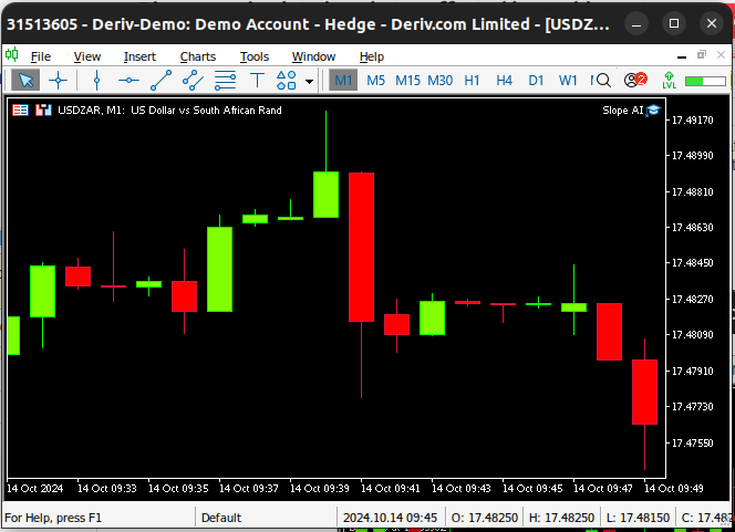
Fig 1: A cluster of Doji Candles

Overview of The Methodology

We analyzed 10 000 rows of M1 Data from the USDZAR pair. The data was fetched from our MetaTrader 5 terminal, using an MQL5 script. We first calculated the slope using the formula we suggested earlier. To calculate the angle of the slope, we used the inverse of the tan trigonometric function, arc-tan. The quantity we calculated displayed dismal correlation levels with our market quotes.

Although our correlation levels were not encouraging, we proceeded to train a selection of 12 different AI models to predict the future value of the USDZAR exchange rate, on 3 groups of input data:

1. OHLC Quotes from our MetaTrader 5 terminal
2. Angle and slope created by price
3. A combination of all 3.

Our best performing model was the simple linear regression, using OHLC. Although it is worth noting that the linear model's accuracy remained the same when we swapped its inputs from group 1 to group 3. None of the models we observed performed better in group 2 than they did in group 1. However, only 2 of the models, we examined, performed best when they used all the available data. The KNeighbors algorithm's performance improved by 20% thanks to our new features. This observation causes us to question what further enhancements we stand to gain, by making other useful transformations to our data.

We successfully tuned the parameters of the KNeighbors model without overfitting the training data and exported our model to ONNX format to be included in our AI powered Expert Advisor.

Fetching The Data We Need

The script below will fetch the data we need from our MetaTrader 5 terminal and save it in CSV format for us. Simply drag and drop the script onto any market you wish to analyze, and you can follow along with us.

//+------------------------------------------------------------------+
//|                                                      ProjectName |
//|                                      Copyright 2020, CompanyName |
//|                                       http://www.companyname.net |
//+------------------------------------------------------------------+
#property copyright "Gamuchirai Zororo Ndawana"
#property link      "https://www.mql5.com/en/users/gamuchiraindawa"
#property version   "1.00"
#property script_show_inputs

//+------------------------------------------------------------------+
//| Script Inputs                                                    |
//+------------------------------------------------------------------+
input int size = 100000; //How much data should we fetch?

//+------------------------------------------------------------------+
//| On start function                                                |
//+------------------------------------------------------------------+
void OnStart()
  {

//--- File name
   string file_name = "Market Data " + Symbol() +".csv";

//--- Write to file
   int file_handle=FileOpen(file_name,FILE_WRITE|FILE_ANSI|FILE_CSV,",");

   for(int i= size;i>=0;i--)
     {
      if(i == size)
        {
         FileWrite(file_handle,"Time","Open","High","Low","Close");
        }

      else
        {
         FileWrite(file_handle,iTime(Symbol(),PERIOD_CURRENT,i),
                   iOpen(Symbol(),PERIOD_CURRENT,i),
                   iHigh(Symbol(),PERIOD_CURRENT,i),
                   iLow(Symbol(),PERIOD_CURRENT,i),
                   iClose(Symbol(),PERIOD_CURRENT,i)
                  );
        }
     }
//--- Close the file
   FileClose(file_handle);

  }
//+------------------------------------------------------------------+

Exploratory Data Analysis

To start our analysis, let us first import the libraries we need.

import numpy as np
import pandas as pd
import seaborn as sns
import matplotlib.pyplot as plt

Now we will read in the market data.

#Read in the data
data = pd.read_csv("Market Data USDZAR.csv")

Our data is arranged in the wrong order, reverse it.

#The data is in reverse order, correct that
data = data[::-1]

Define how far into the future we wish to forecast.

#Define the forecast horizon
look_ahead = 20

Let us apply the slope calculation. Unfortunately, our slope calculations do not always evaluate to a real number. This is one of the limitations of our current version algorithm. Bear in mind, we must arrive at a decision on how we will handle the missing values in our data frame. For now, we will drop all missing values in the data frame.

#Calculate the angle formed by the changes in price, using a ratio of high and low price.
#Then calculate arctan to realize the angle formed by the changes in pirce
data["Slope"] =  (data["Close"] - data["Close"].shift(look_ahead))/(data["Open"] - data["Open"].shift(look_ahead))
data["Angle"] =  np.arctan(data["Slope"])

data.describe()

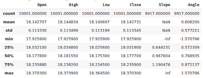
Fig 2: Our data frame after calculating the angle created by price

Let's zoom in on the instances where our slope calculation evaluated to infinity.

data.loc[data["Slope"] == np.inf]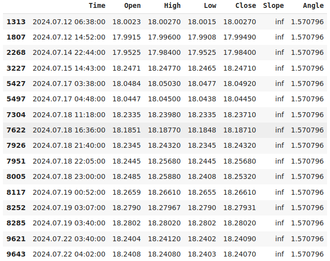

Fig 3: Our records of infinite slope represent instances where the opening price did not change

In the plot below, Fig 4, we randomly selected one of the instances where our slope calculation was infinite. The plot shows that these records map to price fluctuations, whereby the Open price did not change.

pt = 1807
y = data.loc[pt,"Open"]
plt.plot(data.loc[(pt - look_ahead):pt,"Open"])
plt.axhline(y=y,color="red")
plt.xlabel("Time")
plt.ylabel("USDZAR Open Price")
plt.title("A slope of INF means the price has not changed")

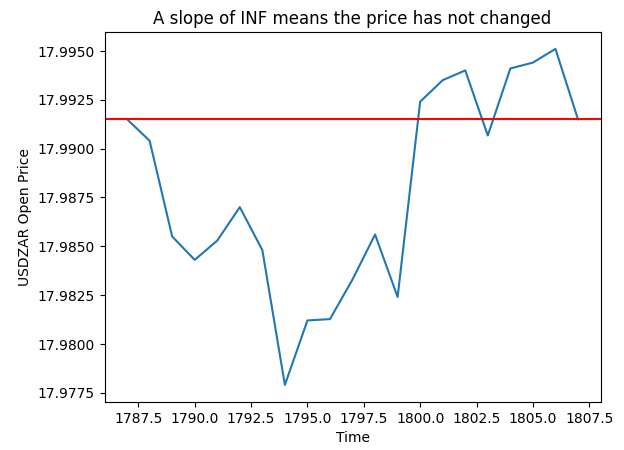
Fig 3: Visualizing the slope values we calculated

For now, we will simplify our discussion by dropping all missing values.

data.dropna(inplace=True)

Now, let us reset the index of our data.

data.reset_index(drop=True,inplace=True)

Let us plot our angle calculations. As we can see from Fig 4 below, our angle calculation revolves around 0, this may give the computer some sense of scale because the further we drift away from 0, the greater the change in price levels.

data.loc[:100,"Angle"].plot()

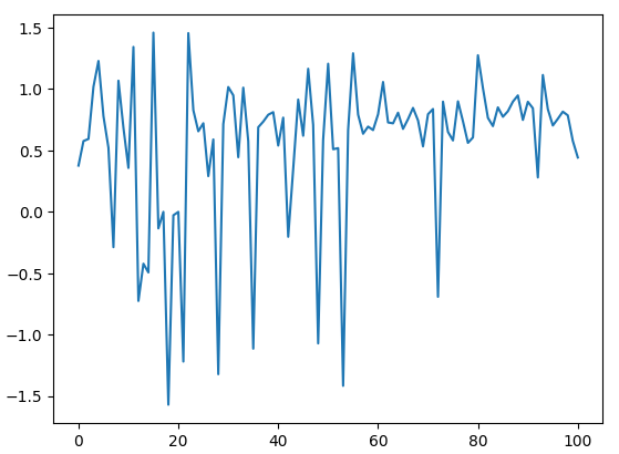
Fig 4: Visualizing the angles created by price changes

Let us now try and estimate the noise in the new feature we have created. We will quantify noise to be the number of times the angle created by price decreased but price levels increased over the same time. This property is undesirable because ideally, we would love a quantity that increases and decreases agreeing with price levels. Unfortunately, our new calculation moves in step with price half of the time, and the other half they may move independently.

To quantify this, we simply counted the number of rows where the slope of the price increased and the future price levels decreased. And we divided this count by the total number of instances where the slope increased. This tells us that, knowing the future value of the slope of the line, tells us very little about the changes in price levels that would have occurred over that same forecast horizon.

#How clean are the signals generated?
1 - (data.loc[(data["Slope"] < data["Slope"].shift(-look_ahead)) & (data["Close"] > data["Close"].shift(-look_ahead))].shape[0] / data.loc[(data["Slope"] < data["Slope"].shift(-look_ahead))].shape[0])

0.51

Exploratory Data Analysis

First, we must define our inputs and outputs.

#Define our inputs and target
ohlc_inputs      = ["Open","High","Low","Close"]
trig_inputs      = ["Angle"]
all_inputs       = ohlc_inputs + trig_inputs
cv_inputs        = [ohlc_inputs,trig_inputs,all_inputs]
target           = "Target"

Now define the classical target, the future price.

#Define the target
data["Target"] = data["Close"].shift(-look_ahead)

Let's also add a few categories to tell our model about the price action that created each candle. If the current candle is the result of a bullish move that happened over the past 20 candles, we will symbolize that with a categorical value set to 1. Otherwise, the value will be set to 0. We will perform the same labeling technique for our angle changes.

#Add a few labels
data["Bull Bear"] = np.nan
data["Angle Up Down"] = np.nan

data.loc[data["Close"] > data["Close"].shift(look_ahead), "Bull Bear"] = 0
data.loc[data["Angle"] > data["Angle"].shift(look_ahead),"Angle Up Down"] = 0
data.loc[data["Close"] < data["Close"].shift(look_ahead), "Bull Bear"] = 1
data.loc[data["Angle"] < data["Angle"].shift(look_ahead),"Angle Up Down"] = 1

Formatting the data.

data.dropna(inplace=True)
data.reset_index(drop=True,inplace=True)
data

Let us analyze the correlation levels in our data. Recall that when we estimated the noise levels associated with the new angle calculation, we observed that price and the angle calculation are only in harmony about 50% of the time. Therefore, the poor correlation levels we observed below in Fig 5 should come as no surprise.

#Let's analyze the correlation levels
sns.heatmap(data.loc[:,all_inputs].corr(),annot=True)

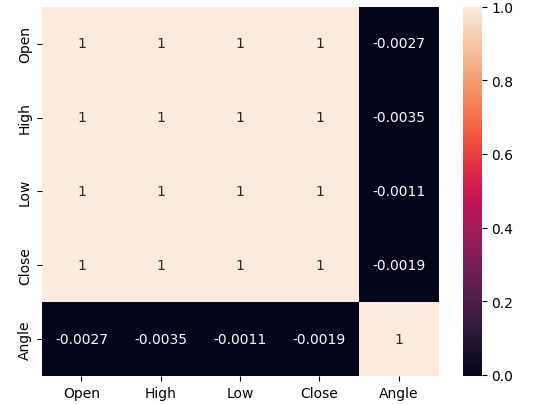
Fig 5: Our angle calculation has very little correlation with any of our price features

Let us also try creating a scatter-plot of the Angle created by price on the x-axis and the Close price on the y-axis. The results obtained are not promising. There is excessive overlap between the instances where price levels fell, the blue dots, and the instances where price levels increased. This makes it challenging for our machine learning models to estimate the mappings between the 2 possible classes of price movements.

sns.scatterplot(data=data,y="Close",x="Angle",hue="Bull Bear")

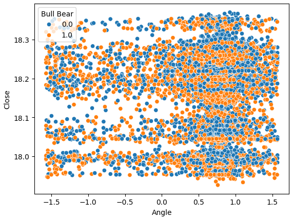
Fig 6: Our Angle calculation is not helping us separate the data better

If we perform a scatter-plot of our 2 engineered features, the Slope and the Angle calculations, against each other, we can clearly observe the non-linear transformation we have applied to the data. Most of our data lies in between the 2 curved ends of the data, and unfortunately, there is no partition between the bullish and bearish price action that may give us an advantage in forecasting future price levels.

sns.scatterplot(data=data,x="Angle",y="Slope",hue="Bull Bear")

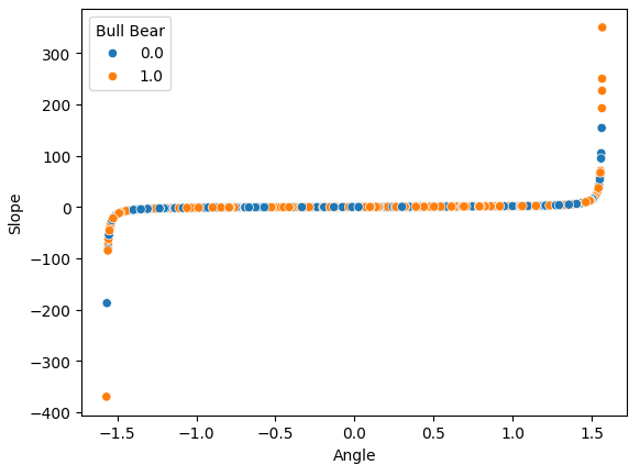
Fig 7: Visualizing our non-linear transformation that we applied to OHLC price data

Let us visualize the noise we estimated at 51% earlier. Let's perform a plot with 2 values on our x-axis. Each value will symbolize whether the angle calculation increased or decreased, respectively. Our y-axis will record the closing price and each of the dots will summarize whether price levels appreciated or depreciated in the same manner that we outlined earlier, blue instances summarize points where future price levels fell.

At first, we estimated the noise, but now we can visualize it. We can clearly see from Fig 8 below, that changes in future price levels appear to have nothing to do with the changes in the angle created by price.

sns.swarmplot(data=data,x="Angle Up Down",y="Close",hue="Bull Bear")

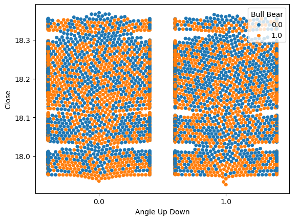
Fig 8: Future price levels appear to have no relationship with the change in the angle

Visualizing the data in 3D shows just how noisy the signal is. We would expect to at least observe a few clusters of points that were all bullish or bearish. However, in this particular instance, we have none. The presence of clusters could possibly identify a pattern that could be interpreted as a trading signal.

#Define the 3D Plot
fig = plt.figure(figsize=(7,7))
ax = plt.axes(projection="3d")
ax.scatter(data["Slope"],data["Angle"],data["Close"],c=data["Bull Bear"])
ax.set_xlabel("Slope")
ax.set_ylabel("Angle")
ax.set_zlabel("Close")

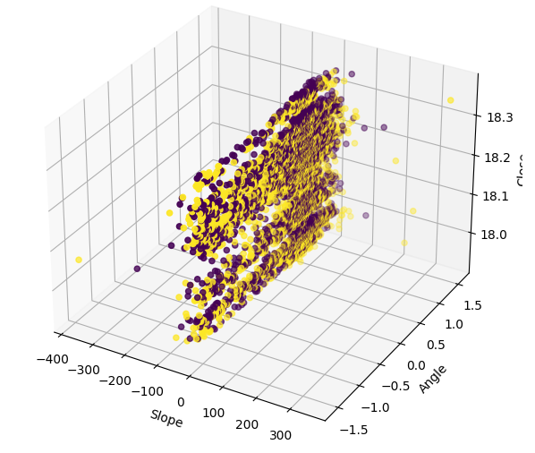
Fig 9: Visualizing our slope data in 3 dimensions

The violin plot allows us to visually compare 2 distributions. The violin plot has a box-plot at its core, to summarize the numerical properties of each distribution. Fig 10 below, gives us hope that the angle calculation is not a waste of time. Each box plot has its average value outlined with a white line. We can clearly see that across both instances of angle movements, the average values of each box-plot were slightly different. While this slight difference may appear insignificant to us as humans, our machine learning models are sensitive enough to pick up and learn from such discrepancies in the distribution of the data.

sns.violinplot(data=data,x="Angle Up Down",y="Close",hue="Bull Bear",split=True)

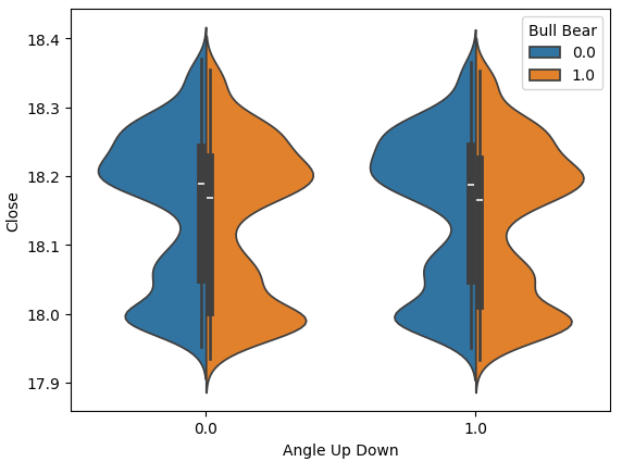
Fig 10: Comparing the distribution of price data between the 2 classes of angle movements

Preparing To Model The Data

Let us now try and model our data. First, we shall import the libraries we need.

from sklearn.model_selection import train_test_split,cross_val_score
from sklearn.preprocessing import StandardScaler
from sklearn.ensemble import RandomForestRegressor, BaggingRegressor, GradientBoostingRegressor,AdaBoostRegressor
from sklearn.svm import LinearSVR
from sklearn.linear_model import LinearRegression, Ridge, Lasso, ElasticNet
from sklearn.neighbors import KNeighborsRegressor
from sklearn.tree import DecisionTreeRegressor
from sklearn.neural_network import MLPRegressor
from sklearn.metrics import mean_squared_error

Split the data into train, test splits.

#Let's split our data into train test splits
train_data, test_data = train_test_split(data,test_size=0.5,shuffle=False)

Scaling the data will help our models learn effectively. Ensure that you only fit the scaler object on the train set, and then transform the test set without fitting the scaler object a second time. Do not fit the scaler object on the entire data set because the parameters learned to scale your data will propagate some information about the future, back into the past.

#Scale the data
scaler = StandardScaler()
scaler.fit(train_data[all_inputs])
train_scaled= pd.DataFrame(scaler.transform(train_data[all_inputs]),columns=all_inputs)
test_scaled = pd.DataFrame(scaler.transform(test_data[all_inputs]),columns=all_inputs)

Define a data-frame to store the accuracy of each model.

#Create a dataframe to store our accuracy in training and testing
columns = [
    "Random Forest",
    "Bagging",
    "Gradient Boosting",
    "AdaBoost",
    "Linear SVR",
    "Linear Regression",
    "Ridge",
    "Lasso",
    "Elastic Net",
    "K Neighbors",
    "Decision Tree",
    "Neural Network"
]
index = ["OHLC","Angle","All"]
accuracy = pd.DataFrame(columns=columns,index=index)

Store the models in a list.

#Store the models
models = [
  RandomForestRegressor(),
  BaggingRegressor(),
  GradientBoostingRegressor(),
  AdaBoostRegressor(),
  LinearSVR(),
  LinearRegression(),
  Ridge(),
  Lasso(),
  ElasticNet(),
  KNeighborsRegressor(),
  DecisionTreeRegressor(),
  MLPRegressor(hidden_layer_sizes=(4,6))
]

Cross-validate each model.

#Cross validate the models
#First we have to iterate over the inputs
for k in np.arange(0,len(cv_inputs)):
  current_inputs = cv_inputs[k]
  #Then fit each model on that set of inputs
  for i in np.arange(0,len(models)):
    score = cross_val_score(models[i],train_scaled[current_inputs],train_data[target],cv=5,scoring="neg_mean_squared_error",n_jobs=-1)
    accuracy.iloc[k,i] = -score.mean()

We tested the models using 3 sets of inputs:

1. Just the OHLC prices.
2. Just the slope and angle created.
3. All the data we had.

Not all our models were able to effectively use our features. From the 12 models in our pool of candidates, the KNeighbors model gained a 20% improvement in performance from our new features and was clearly the best model we had at this point.

While our linear regression is the best model from the entire pool, this demonstration suggests that there may be other transformations we are simply not aware of that could lower our accuracy levels even further.

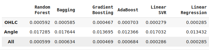
Fig 11: Some of our accuracy levels. Note that only 2 of our models demonstrated skill using the new features we have engineered.

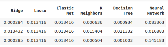
Fig 12: AdaBoost and KNeighbors were our most promising models, we decided to optimize the KNeighbors model

Deeper Optimization

Let us try and find better settings for our indicator than the default settings it comes with.

from sklearn.model_selection import RandomizedSearchCV

Create instances of our model.

model = KNeighborsRegressor(n_jobs=-1)

Define the tuning parameters.

tuner = RandomizedSearchCV(model,
  {
    "n_neighbors": [2,3,4,5,6,7,8,9,10],
    "weights": ["uniform","distance"],
    "algorithm": ["auto","ball_tree","kd_tree","brute"],
    "leaf_size": [1,2,3,4,5,10,20,30,40,50,60,100,200,300,400,500,1000],
    "p": [1,2]
  },
    n_iter = 100,
    n_jobs=-1,
    cv=5
)

Fit the tuner object.

tuner.fit(train_scaled.loc[:,all_inputs],train_data[target])

The best parameters we have found.

tuner.best_params_

{'weights': 'uniform',
 'p': 1,
 'n_neighbors': 10,
 'leaf_size': 100,
 'algorithm': 'ball_tree'}

Our best score on the training set was 71%. We, don't really care much about the training errors. We are more concerned with how well our model will generalize to new data.

tuner.best_score_

0.7106899297793474

Testing For Overfitting

Let us see if we were overfitting to the training set. Overfitting happens when our model learns meaningless information from our training set. There are various ways we can test if we are overfitting, One way is to compare the customized model, against a model that has no prior knowledge about the data.

#Testing for over fitting
model = KNeighborsRegressor(n_jobs=-1)

custom_model = KNeighborsRegressor(n_jobs=-1,weights= 'uniform',p=1,n_neighbors= 10,leaf_size= 100,algorithm='ball_tree')

If we fail to outperform a default instance of the model, we can be confident we may have over customized our model to the training set. We can clearly see that we outperformed the default model, which is good news.

model.fit(train_scaled.loc[:,all_inputs],train_data[target])
custom_model.fit(train_scaled.loc[:,all_inputs],train_data[target])

Default Model	Customized Model
0.0009797322460441842	0.0009697248896608824

Exporting To ONNX

Open Neural Network Exchange (ONNX) is an open-source protocol for building and sharing machine learning models in a model agnostic manner. We will utilize the ONNX API to export our AI model from Python and import it into an MQL5 program.

First, we need to apply transformations to our price data that we can always reproduce in MQL5. Let us save the mean and standard deviation values of each column into a CSV file.

data.loc[:,all_inputs].mean().to_csv("USDZAR M1 MEAN.csv")
data.loc[:,all_inputs].std().to_csv("USDZAR M1 STD.csv")

Now apply the transformation on the data.

data.loc[:,all_inputs] = ((data.loc[:,all_inputs] - data.loc[:,all_inputs].mean())/ data.loc[:,all_inputs].std())

Now let us import the libraries we need.

import onnx
from skl2onnx import convert_sklearn
from skl2onnx.common.data_types import FloatTensorType

Define the input type of our model.

#Define the input shape
initial_type = [('float_input', FloatTensorType([1, len(all_inputs)]))]

Fit the model on all the data we have.

#Fit the model on all the data we have
custom_model.fit(data.loc[:,all_inputs],data.loc[:,"Target"])

Convert the model to ONNX format and save it.

#Convert the model to ONNX format
onnx_model = convert_sklearn(model, initial_types=initial_type,target_opset=12)
#Save the ONNX model
onnx.save(onnx_model,"USDZAR M1 OHLC Angle.onnx")

Building Our Expert Advisor in MQL5

Let us now integrate our AI model into a trading application, so we can trade with an edge over the market. Our trading strategy will use our AI Model to detect the trend on the M1. We will seek additional confirmation from the performance of the USADZAR pair on the daily time frame. If our AI model is detecting an uptrend, we will want to see bullish price action on the daily chart. Additionally, we will also want further confirmation from the Dollar Index. Following our example of buying on the M1, we will also need to observe bullish price action on the Dollar Index daily chart as a sign that the Dollar is likely to continue to rally on bigger time frames.

First, we need to import the ONNX model we have just created.

//+------------------------------------------------------------------+
//|                                                     Slope AI.mq5 |
//|                                        Gamuchirai Zororo Ndawana |
//|                          https://www.mql5.com/en/gamuchiraindawa |
//+------------------------------------------------------------------+
#property copyright "Gamuchirai Zororo Ndawana"
#property link      "https://www.mql5.com/en/gamuchiraindawa"
#property version   "1.00"

//+------------------------------------------------------------------+
//| Load the ONNX files                                              |
//+------------------------------------------------------------------+
#resource "\\Files\\USDZAR M1 OHLC Angle.onnx" as  const uchar onnx_buffer[];

Let us also load our trade library for managing our open positions.

//+------------------------------------------------------------------+
//| Libraries                                                        |
//+------------------------------------------------------------------+
#include <Trade\Trade.mqh>
CTrade Trade;

Define a few global variables that we will need.

//+------------------------------------------------------------------+
//| Global variables                                                 |
//+------------------------------------------------------------------+
double mean_values[5] = {18.143698,18.145870,18.141644,18.143724,0.608216};
double std_values[5] = {0.112957,0.113113,0.112835,0.112970,0.580481};
long   onnx_model;
int    macd_handle;
int    usd_ma_slow,usd_ma_fast;
int    usd_zar_slow,usd_zar_fast;
double macd_s[],macd_m[],usd_zar_s[],usd_zar_f[],usd_s[],usd_f[];
double bid,ask;
double vol = 0.3;
double profit_target = 10;
int    system_state = 0;
vectorf model_forecast = vectorf::Zeros(1);

We have now arrived at the initialization procedure for our trading application. For now, all we need is to load our ONNX model and technical indicators.

//+------------------------------------------------------------------+
//| Expert initialization function                                   |
//+------------------------------------------------------------------+
int OnInit()
  {
//--- Load the ONNX file
   if(!onnx_load())
     {
      //--- We failed to load the ONNX file
      return(INIT_FAILED);
     }

//--- Load the MACD Indicator
   macd_handle  = iMACD("EURUSD",PERIOD_CURRENT,12,26,9,PRICE_CLOSE);
   usd_zar_fast = iMA("USDZAR",PERIOD_D1,20,0,MODE_EMA,PRICE_CLOSE);
   usd_zar_slow = iMA("USDZAR",PERIOD_D1,60,0,MODE_EMA,PRICE_CLOSE);
   usd_ma_fast  = iMA("DXY_Z4",PERIOD_D1,20,0,MODE_EMA,PRICE_CLOSE);
   usd_ma_slow  = iMA("DXY_Z4",PERIOD_D1,60,0,MODE_EMA,PRICE_CLOSE);

//--- Everything went fine
   return(INIT_SUCCEEDED);
  }

If our program is no longer in use, let us free up the resources it was using.

//+------------------------------------------------------------------+
//| Expert deinitialization function                                 |
//+------------------------------------------------------------------+
void OnDeinit(const int reason)
  {
//--- Release the handles don't need
   OnnxRelease(onnx_model);
   IndicatorRelease(macd_handle);
   IndicatorRelease(usd_zar_fast);
   IndicatorRelease(usd_zar_slow);
   IndicatorRelease(usd_ma_fast);
   IndicatorRelease(usd_ma_slow);
  }

Whenever we receive updated prices, let us store our new market data, fetch a new prediction from our model and then decide if we need to look for a position in the market, or close the positions we have.

//+------------------------------------------------------------------+
//| Expert tick function                                             |
//+------------------------------------------------------------------+
void OnTick()
  {
//--- Update our market data
   update();
//--- Get a prediction from our model
   model_predict();

   if(PositionsTotal() == 0)
     {
      find_entry();
     }

   if(PositionsTotal() > 0)
     {
      manage_positions();
     }
  }
//+------------------------------------------------------------------+

The function that actually updates our market data is defined below. We are relying on the CopyBuffer command to fetch the current value of each indicator into its array buffer. We will use these moving average indicators for trend confirmation.

//+------------------------------------------------------------------+
//| Update our market data                                           |
//+------------------------------------------------------------------+
void update(void)
  {
   bid = SymbolInfoDouble(Symbol(),SYMBOL_BID);
   ask = SymbolInfoDouble(Symbol(),SYMBOL_ASK);

   CopyBuffer(macd_handle,0,0,1,macd_m);
   CopyBuffer(macd_handle,1,0,1,macd_s);
   CopyBuffer(usd_ma_fast,0,0,1,usd_f);
   CopyBuffer(usd_ma_slow,0,0,1,usd_s);
   CopyBuffer(usd_zar_fast,0,0,1,usd_zar_f);
   CopyBuffer(usd_zar_slow,0,0,1,usd_zar_s);
  }
//+------------------------------------------------------------------+

Not only that, but we need to define how exactly our model is going to make forecasts. Additionally, let us start by first calculating the angle formed by price fluctuations, and then we will store our model inputs into a vector. Finally, we will standardize and scale our model inputs before calling the OnnxRun function to obtain a forecast from our AI model.

//+------------------------------------------------------------------+
//| Get a forecast from our model                                    |
//+------------------------------------------------------------------+
void model_predict(void)
  {
   float angle = (float) MathArctan(((iOpen(Symbol(),PERIOD_M1,1) - iOpen(Symbol(),PERIOD_M1,20)) / (iClose(Symbol(),PERIOD_M1,1) - iClose(Symbol(),PERIOD_M1,20))));
   vectorf model_inputs = {(float) iOpen(Symbol(),PERIOD_M1,1),(float) iHigh(Symbol(),PERIOD_M1,1),(float) iLow(Symbol(),PERIOD_M1,1),(float) iClose(Symbol(),PERIOD_M1,1),(float) angle};
   for(int i = 0; i < 5; i++)
     {
      model_inputs[i] = (float)((model_inputs[i] - mean_values[i])/std_values[i]);
     }
//--- Log
   Print("Model inputs: ");
   Print(model_inputs);

   if(!OnnxRun(onnx_model,ONNX_DATA_TYPE_FLOAT,model_inputs,model_forecast))
     {
      Comment("Failed to obtain a forecast from our model: ",GetLastError());
     }

  }

The following function will load our ONNX model from the ONNX buffer we defined earlier.

//+------------------------------------------------------------------+
//| ONNX Load                                                        |
//+------------------------------------------------------------------+
bool onnx_load(void)
  {
//--- Create the ONNX model from the buffer we defined
   onnx_model = OnnxCreateFromBuffer(onnx_buffer,ONNX_DEFAULT);

//--- Define the input and output shapes
   ulong input_shape[] = {1,5};
   ulong output_shape[] = {1,1};

//--- Validate the I/O parameters
   if(!(OnnxSetInputShape(onnx_model,0,input_shape))||!(OnnxSetOutputShape(onnx_model,0,output_shape)))
     {
      //--- We failed to define the I/O parameters
      Comment("[ERROR] Failed to load AI Model Correctly: ",GetLastError());
      return(false);
     }

//--- Everything was okay
   return(true);
  }

Additionally, our system needs rules on when it should close our positions. If the floating profit on our current positions is greater than our profit target, we will close our positions. Otherwise, if the system changes state, then we will close our positions accordingly.

//+------------------------------------------------------------------+
//| Manage our open positions                                        |
//+------------------------------------------------------------------+
void manage_positions(void)
  {
   if(PositionSelectByTicket(PositionGetTicket(0)))
     {
      if(PositionGetDouble(POSITION_PROFIT) > profit_target)
        {
         Trade.PositionClose(Symbol());
        }
     }

   if(system_state == 1)
     {
      if(macd_m[0] < macd_s[0])
        {
         if(model_forecast[0] < iClose(Symbol(),PERIOD_M1,0))
           {
            Trade.PositionClose(Symbol());
           }
        }
     }

   if(system_state == -1)
     {
      if(macd_m[0] > macd_s[0])
        {
         if(model_forecast[0] > iClose(Symbol(),PERIOD_M1,0))
           {
            Trade.PositionClose(Symbol());
           }
        }
     }
  }

The following function is responsible for opening our positions. We will only open a buy position if:

1. The MACD main line is above the signal
2. Our AI forecast is greater than the current close
3. The Dollar index and the USDZAR pair are both demonstrating bullish price action on the Daily chart.

The opposite is also true for determining our sell positions. We can only open a position of all our conditions are satisfied simultaneously, otherwise our system will wait.

//+------------------------------------------------------------------+
//| Find an entry                                                    |
//+------------------------------------------------------------------+
void find_entry(void)
  {
   if(macd_m[0] > macd_s[0])
     {
      if(model_forecast[0] > iClose(Symbol(),PERIOD_M1,0))
        {
         if((usd_f[0] > usd_s[0]) && (usd_zar_f[0] > usd_zar_s[0]))
           {
            Trade.Buy(vol,Symbol(),ask,0,0,"Slope AI");
            system_state = 1;
           }
        }
     }

   if(macd_m[0] < macd_s[0])
     {
      if(model_forecast[0] < iClose(Symbol(),PERIOD_M1,0))
        {
         if((usd_f[0] < usd_s[0]) && (usd_zar_f[0] < usd_zar_s[0]))
           {
            Trade.Sell(vol,Symbol(),bid,0,0,"Slope AI");
            system_state = -1;
           }
        }
     }
  }

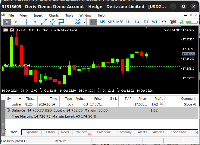
Fig 12: Our AI system in action

Conclusion

So far, we have demonstrated that there are still some obstacles that stand in the way of traders that may wish to use the slope formed by price action into their trading strategies. However, it appears that any effort applied in this direction may be worth the time invested. Exposing the relationship between price levels by using the slope improved our KNeighbors model's performance by 20%, this calls us to question just how much more performance gains we stand to realize if we keep searching in this direction. Additionally, it also highlights that each model probably has its own specific set of transformations that will enhance its performance, our job now becomes to realize this mapping.