
Feature Engineering With Python And MQL5 (Part I): Forecasting Moving Averages For Long-Range AI Models

When applying AI to any task, we must try our best to give the model as much useful information about the real world as we can. To describe different properties of the market to our AI models, we must manipulate and transform the input data, this process is referred to as feature engineering. This series of articles will teach you how to transform your market data, to reduce the error levels of your models. Today, I will focus on how to use moving averages to increase the forecasting range of your AI models in a fashion that gives complete control and a reasonable understanding of the global effectiveness of the strategy.
Overview of The Strategy
The last we spoke of forecasting moving averages with AI, I provided evidence that suggested the moving average values are easier for our AI models to predict than future price levels, the link to that article is provided here. However, for us to be confident that our findings are significant, I trained 2 identical AI models on more than 200 different market symbols and compared the accuracy of forecasting price against the accuracy of forecasting the moving average and the results appear to show that our accuracy levels drop on average by 34% if we forecast price over of the moving averages.
On average, we can expect 70% accuracy when forecasting the moving averages, compared to an expectation of 52% accuracy when forecasting price. We are all aware that, depending on your period, the moving average indicator does not follow price levels very closely, for example, price may fall over 20 candles while the moving averages are rising over the same interval. This divergence is undesirable for us because it is possible for us to predict the moving average future direction correctly, but price may diverge. Remarkably, we observed that the rate of divergence remains fixed around 31% across all markets, and our ability to forecast divergences averaged at 68%.
Additionally, the variance of our ability to forecast divergence and the occurrence of divergence was 0.000041 and 0.000386 respectively. This shows that our model is capable of correcting itself with a reliable level of skill. Members of the community looking to apply AI into long-term trading strategies should consider this alternative approach on higher time frames. Our discussion is limited to the M1 for now because this time frame ensures we will have sufficient data across all 297 markets so we can make fair comparisons.
There are many possible reasons why the moving averages are easier to predict than the price itself. This may be true because predicting moving averages is more inline with the idea of linear regression, than predicting price is, namely Linear regression assumes the data is a linear combination (sum) of several inputs: Moving averages are a summation off previous price values, this means the linear assumption is true. Price itself is not a simple summation of real-world variables, it is a complex relation between many variables.
Getting Started
We will first need to import our standard libraries for scientific computing in Python.
#Load the libraries we need
import pandas as pd
import numpy as np
import MetaTrader5 as mt5
from sklearn.model_selection import TimeSeriesSplit,cross_val_score
from sklearn.linear_model import LogisticRegression,LinearRegression
import matplotlib.pyplot as plt
Let us initialize our MetaTrader 5 terminal.
#Initialize the terminal
mt5.initialize() How many symbols do we have available?
#The total number of symbols we have
print(f"Total Symbols Available: ",mt5.symbols_total())
Get the names of all symbols.
#Get the names of all pairs
symbols = mt5.symbols_get()
idx = [s.name for s in symbols]
Create a data frame to store our accuracy levels on all symbols.
global_params = pd.DataFrame(index=idx,columns=["OHLC Error","MAR Error","Noise Levels","Divergence Error"])
global_params
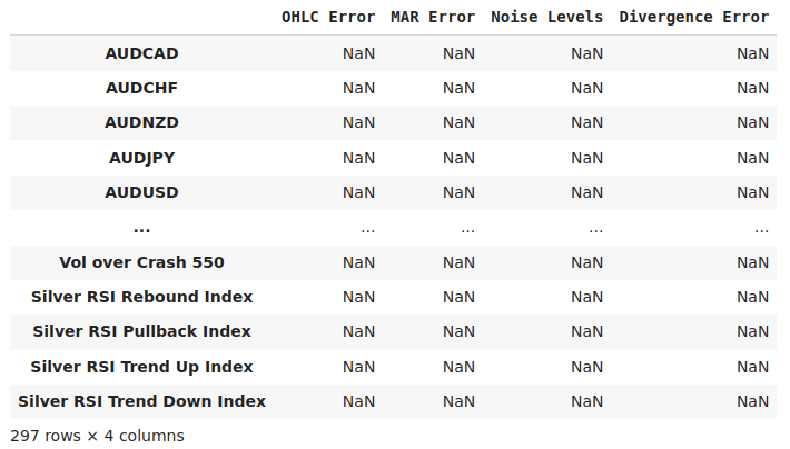
Fig 1: Our data frame that will store our accuracy levels across all markets in our terminal
Define our time-series split object.
#Define the time series split object
tscv = TimeSeriesSplit(n_splits=5,gap=10)
Measure our accuracy on all symbols.
#Iterate over all symbols
for i in np.arange(global_params.dropna().shape[0],len(idx)):
    #Fetch M1 Data
    data = pd.DataFrame(mt5.copy_rates_from_pos(cols[i],mt5.TIMEFRAME_M1,0,50000))
    data.rename(columns={"open":"Open","high":"High","low":"Low","close":"Close"},inplace=True)
    #Define our period
    period = 10
    #Add the classical target
    data.loc[data["Close"].shift(-period) > data["Close"],"OHLC Target"] = 1
    #Calculate the returns
    data.loc[:,["Open","High","Low","Close"]] = data.loc[:,["Open","High","Low","Close"]].diff(period)
    data["RMA"] = data["Close"].rolling(period).mean()
    #Calculate our new target
    data.dropna(inplace=True)
    data.reset_index(inplace=True,drop=True)
    data.loc[data["RMA"].shift(-period) > data["RMA"],"New Target"] = 1
    data = data.iloc[0:-period,:]
    #Calculate the divergence target
    data.loc[data["OHLC Target"] != data["New Target"],"Divergence Target"] = 1
    #Noise ratio
    global_params.iloc[i,2] = data.loc[data["New Target"] != data["OHLC Target"]].shape[0] / data.shape[0]
    #Test our accuracy predicting the future close price
    score = cross_val_score(LogisticRegression(),data.loc[:,["Open","High","Low","Close"]],data["OHLC Target"],cv=tscv)
    global_params.iloc[i,0] = score.mean()
    #Test our accuracy predicting the moving average of future returns
    score = cross_val_score(LogisticRegression(),data.loc[:,["Open","Close","RMA"]],data["New Target"],cv=tscv)
    global_params.iloc[i,1] = score.mean()
    #Test our accuracy predicting the future divergence between price and its moving average
    score = cross_val_score(LogisticRegression(),data.loc[:,["Open","Close","RMA"]],data["Divergence Target"],cv=tscv)
    global_params.iloc[i,3] = score.mean()
    print(f"{((i/len(idx)) * 100)}% complete")

#We are done
print("Done")
Done
Analyzing The Results
Now that we have fetched our market data and assessed our model on the 2 targets, let us now summarize the results of our test across all markets. We will start by summarizing our accuracy predicting the change in the future close price. Fig 2 below shows the summary of predicting the change in future close price. The red horizontal line represents the 50% accuracy threshold. Our average accuracy using this technique is denoted by the blue horizontal line. As we can see, our average accuracy is not significantly far from the 50% threshold, this is not encouraging information.
However, to be fair, we can also observe that some markets in particular are well above the average, and can be predicted with more than 65% accuracy. This is impressive, but it also warrants further investigation to determine if the results are meaningful, or they could've happened by chance.
global_params.iloc[:,0].plot()
plt.title("OHLC Accuracy")
plt.xlabel("Market")
plt.ylabel("5-fold Accuracy %")
plt.axhline(global_params.iloc[:,0].mean(),linestyle='--')
plt.axhline(0.5,linestyle='--',color='red') 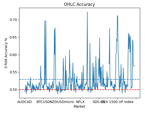
Fig 2: Our average accuracy predicting price
Let us now turn our attention to our accuracy predicting the change in the moving-averages. Fig 3 below summarizes the data for us. Again, the red line represents the 50% threshold, the gold line represents our average accuracy predicting changes in price levels and the blue line is our average accuracy predicting changes in the moving average. To simply say that our model is better at predicting the moving averages, is an understatement. I think it is no longer a subject of debate, but simply a matter of fact, that our models are better at predicting certain indicators than they are at predicting price.
global_params.iloc[:,1].plot()
plt.title("Moving Average Returns Accuracy")
plt.xlabel("Market")
plt.ylabel("5-fold Accuracy %")
plt.axhline(global_params.iloc[:,1].mean(),linestyle='--')
plt.axhline(global_params.iloc[:,0].mean(),linestyle='--',color='orange')
plt.axhline(0.5,linestyle='--',color='red') 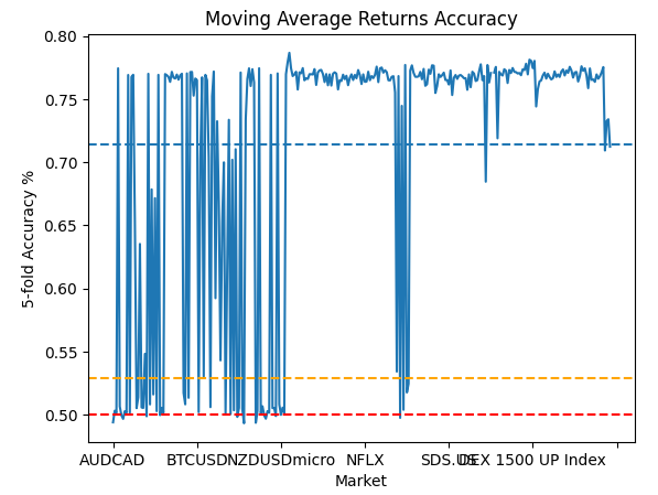
Fig 3: Our accuracy predicting the change in the moving average
Let us now observe the rate at which price and the moving average diverge. Divergence levels close to 50% are bad because that means we cannot be reasonably certain if the price and the moving average are going to move together, or in opposite directions. Fortunately for us, the noise levels appeared constant across all the markets we evaluated. The noise levels varied between 35% and 30%.
global_params.iloc[:,2].plot()
plt.title("Noise Level")
plt.xlabel("Market")
plt.ylabel("Percentage of Divergence:Price And Moving Average")
plt.axhline(global_params.iloc[:,2].mean(),linestyle='--') 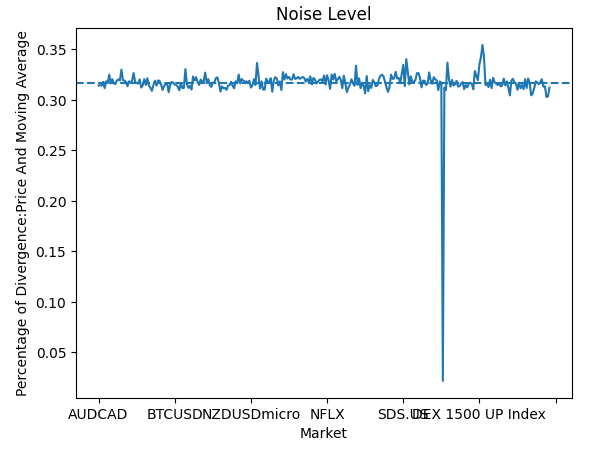
Fig 4: Visualizing our noise levels across all markets
If two variables have a ratio that is almost constant, then it may be a sign that there is a relationship we can model. Let us observe how well we can forecast divergence between price and the moving average. Our rationale is simple, if our model forecasts that the moving average will fall, can we reasonably predict if price will move in the same direction, or if price will diverge from the moving average? It turns out, we can predict divergence with a reliable level of accuracy, almost 70% on average.
global_params.iloc[:,3].plot()
plt.title("Divergence Accuracy")
plt.xlabel("Market")
plt.ylabel("5-fold Accuracy %")
plt.axhline(global_params.iloc[:,3].mean(),linestyle='--') 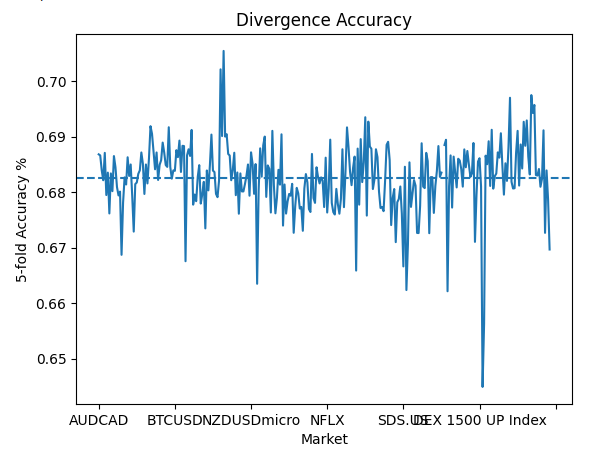
Fig 5: Our accuracy predicting divergence between price and the moving average
We can also summarize our findings into tabular form. So we can easily compare our accuracy levels between the market returns and a moving average of the returns. Note that, even though our moving average may "lag" behind price, our accuracy predicting reversals is still significantly greater than our accuracy predicting price itself.
| Metric | Accuracy |
|---|---|
| Returns Error | 0.525353 |
| Moving Average of Returns Error | 0.705468 |
| Noise Levels | 0.317187 |
| Divergence Error | 0.682069 |
Let's see which markets our model performed best on.
global_params.sort_values("MAR Error",ascending=False) 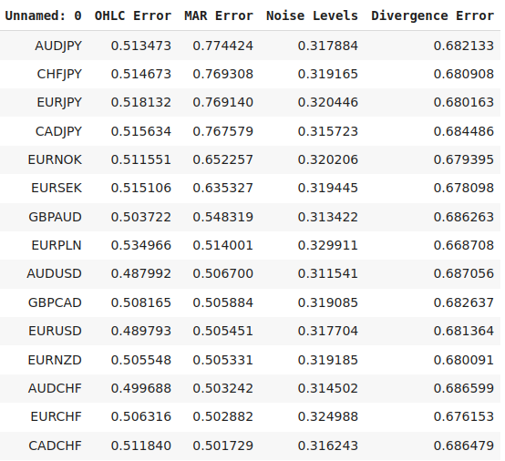
Fig 6: Our best performing markets
Optimizing For Our Best Performing Market
Let us now engineer our and tailor our moving average indicator for one of the market in which our performance is greatest. We will also visually compare our new engineered feature against the classical features. We will start by specifying our selected market.
symbol = "AUDJPY" Ensure we can reach the terminal.
#Reach the terminal
mt5.initialize() Now, fetch market data.
data = pd.DataFrame(mt5.copy_rates_from_pos(symbol,mt5.TIMEFRAME_D1,365*2,5000))
Importing the libraries we need.
#Standard libraries
import seaborn                 as     sns
from   mpl_toolkits.mplot3d    import Axes3D
from   sklearn.linear_model    import LinearRegression
from   sklearn.neural_network  import MLPRegressor
from   sklearn.metrics         import mean_squared_error
from   sklearn.model_selection import cross_val_score,TimeSeriesSplit
Define the start and end point for our period calculation and our forecast horizon. Ensure that both inputs are of the same dimension, otherwise our code will break.
#Define the input range
x_min , x_max = 2,100 #Look ahead
y_min , y_max = 2,100 #Period
Sample our input domain in steps of 5 so that our calculations are detailed and inexpensive to obtain.
#Sample input range uniformly
x_axis = np.arange(x_min,x_max,2) #Look ahead
y_axis = np.arange(y_min,y_max,2) #Period
Create a mesh-grid using our x_axis and y_axis. The mesh-grid is composed of 2, 2-dimensional arrays that define all possible combinations of periods of forecast horizons we wish to evaluate.
#Create a meshgrid
x , y = np.meshgrid(x_axis,y_axis)
Next, we need a function that is going to fetch our market data and label it for us to evaluate.
def clean_data(look_ahead,period):
    #Fetch the data from our terminal and clean it up
    data = pd.DataFrame(mt5.copy_rates_from_pos('AUDJPY',mt5.TIMEFRAME_D1,365*2,5000))
    data['time'] = pd.to_datetime(data['time'],unit='s')
    data['MA'] = data['close'].rolling(period).mean()
    #Transform the data
    #Target
    data['Target'] = data['MA'].shift(-look_ahead) - data['MA']
    #Change in price
    data['close']  = data['close'] - data['close'].shift(period)
    #Change in MA
    data['MA']  = data['MA'] - data['MA'].shift(period)
    data.dropna(inplace=True)
    data.reset_index(drop=True,inplace=True)
    return(data)
The following function will perform 5-fold cross validation on our AI model.
#Evaluate the objective function
def evaluate(look_ahead,period):
    #Define the model
    model = LinearRegression()
    #Define our time series split
    tscv = TimeSeriesSplit(n_splits=5,gap=look_ahead)
    temp = clean_data(look_ahead,period)
    score = np.mean(cross_val_score(model,temp.loc[:,["Open","High","Low","Close"]],temp["Target"],cv=tscv))
    return(score)
Finally, our objective function. Our objective function is simply the 5-fold validation error of our model under the new settings we wish to evaluate. Recall we are trying to find the optimal distance into the future our model should forecast, and additionally, we are trying to locate the period with which we should calculate changes in price.
#Define the objective
def objective(x,y):
    #Define the output matrix
    results = np.zeros([x.shape[0],y.shape[0]])
    #Fill in the output matrix
    for i in np.arange(0,x.shape[0]):
        #Select the rows
        look_ahead = x[i]
        period     = y[i]
        for j in np.arange(0,y.shape[0]):
            results[i,j] = evaluate(look_ahead[j],period[j])
    return(results)
We will evaluate our model's relationship with the market as we attempt to predict the change in price levels directly. Fig 7 shows the relationship between our model and the change in price, whilst Fig 8 shows the relationship between our model and the change in the moving average. The white dot in both plots symbolizes the combination of inputs that resulted in the lowest error for us.
res = objective(x,y)
res = np.abs(res)
Plotting our model's best performance predicting the AUDJPY Daily return. The data is revealing that when we are forecasting the future changes in price, the best we can do forecast 1 step into the future. Human traders do not simply look 1 step ahead when they place their trades. So the results we have obtained by forecasting market returns directly, limit our approach and make our models fixated on the next candle.
plt.contourf(x,y,res,100,cmap="jet")
plt.plot(x_axis[res.min(axis=0).argmin()],y_axis[res.min(axis=1).argmin()],'.',color='white')
plt.ylabel("Differencing Period")
plt.xlabel("Forecast Horizon")
plt.title("Linear Regression Accuracy Forecasting AUDJPY Daily Return") 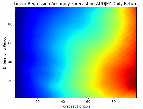
Fig 7:Visualizing our model's capability of forecasting future price levels
Once we start forecasting the change in the moving average as opposed to the change in price, we can observe that our optimal forecast horizon shifts to the right. Fig 8 below, shows that by forecasting the change in the moving averages, we can now reliably forecast 22 steps into the future, as opposed to 1 step into the future when forecasting the change in price.
plt.contourf(x,y,res,100,cmap="jet")
plt.plot(x_axis[res.min(axis=0).argmin()],y_axis[res.min(axis=1).argmin()],'.',color='white')
plt.ylabel("Differencing Period")
plt.xlabel("Forecast Horizon")
plt.title("Linear Regression Accuracy Forecasting AUDJPY Daily Moving Average Return") 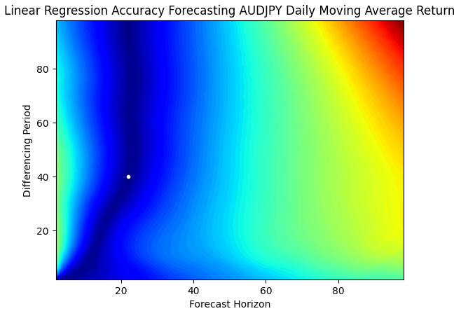
Fig 8:Visualizing our model's capability of forecasting future moving average levels
What's even more impressive is that at the optimal points, our error levels on the two targets were identical. In other words, it is just as easy for our model to predict the change in the moving average 40 steps into the future, as it is for our model to predict the change in price 1 step into the future. Therefore, the moving average prediction gives us greater range, without increasing the error of our predictions.
When we visualize the results of our test in 3D, the difference between the 2 targets becomes clear. Fig 9 below, shows us the relationship between the changes in price levels and the forecasting parameters for our model. There is a clear trend we can see from the data, as we forecast further into the future, our results get worse. Therefore, when we design our AI models this way, they are somewhat "short-sighted" and cannot reasonably forecast intervals larger than 20.
Fig 10, was created from the relationship between our model and its error when forecasting the changes in the moving averages. The surface plot exhibits desirable properties, we can clearly see that as we forecast further into the future and increase the period of calculating the change in the moving average, our error rates fall smoothly to a minimum low and then start to rise again. This visual demonstration shows how much easier it is for our model to predict the moving average as compared to predicting price.
#Create a surface plot
fig , ax = plt.subplots(subplot_kw={"projection":"3d"})
fig.set_size_inches(8,8)
ax.plot_surface(x,y,optimal_nn_res,cmap="jet")
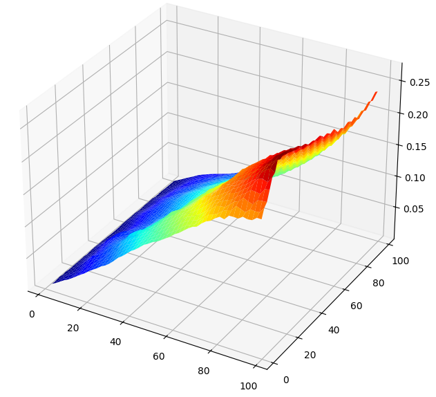
Fig 9: Visualizing the relationship between our model and the changes in the Daily price of the AUDJPY.
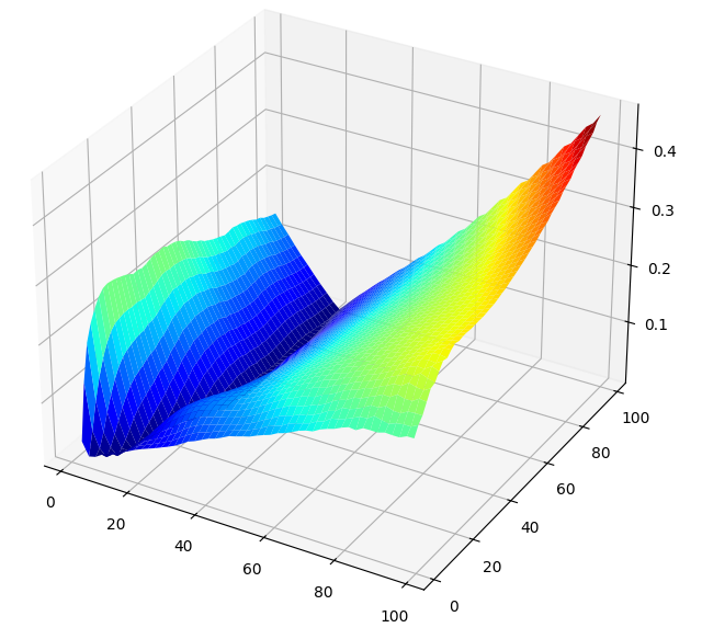
Fig 10: The relationship between our model and the changes to the moving average value on the AUDJPY pair.
Non-Linear Transformations: Wavelet Denoising
So far, we have only applied linear transformations to our data. We can search even deeper and apply non-linear transformations to the model's input data. Feature engineering is at times simply a process of trail and error. We are not always guaranteed to obtain better results. Therefore, we apply these transformations in an ad-hoc manner, we do not have a precise formula to show us the "best" transformation we should apply at any given moment.
The wavelet transformation is a mathematical tool used to create a frequency and time representation of data. It is commonly used in signal and image processing tasks to separate the noise from the signal we are trying to process. After the transformation has been applied, our data will be in the frequency domain. The idea is that, the noise in our data is coming from the small frequency values identified by the transformation. All values, below a certain threshold, are shrunk to 0 in one of 2 possible ways. The result is a sparse representation of the original data.
Wavelet denoising has several advantages over other popular techniques, such as the Fast Fourier Transformation (FFT). For readers who may be unfamiliar, the Fourier Transformation represents any signal as a summation of sine and cosine waves. Unfortunately, the Fourier Transformation filters our high frequency-values. This may not always be desirable, especially for data where the signal is in the high-frequency domain. Given that we are uncertain whether our signal is in the high or low-frequency domain, we need a transformation that is flexible enough to perform this task in an unsupervised way. The wavelet transform will preserve the signal in the data, while filtering out as much of the noise as possible.
To follow along with us, ensure you have installed scikit learn image and its dependency PyWavelets. For readers who wish to create a complete trading application in MQL5, implementing and debugging the transformation from scratch may prove too involving. It is easier for us to progress without it. And for readers that may desire to interface with the terminal using the Python library, the transformation is a tool worth including in your arsenal.
We can compare the change in validation accuracy to see if the transformation is helping our model, and it is. Note, we only apply the transformation to the model's inputs and not the target, we preserve the target. Observe that our validation accuracy indeed fell. We are using the wavelet transformation with a hard threshold, so it sets all noise coefficients to 0. Alternatively, we could use a soft threshold, which would direct our noise coefficients to 0 but may not set them exactly at 0.
#Benchmark Score
np.mean(cross_val_score(LinearRegression(),data.loc[:,["MA"]],data["Target"]))
#Wavelet denoising
data["Denoised"] = denoise_wavelet(
    data["MA"],
    method='BayesShrink',
    mode='hard',
    rescale_sigma=True,
    wavelet_levels = 3,
    wavelet='sym5'
    )
np.mean(cross_val_score(LinearRegression(),np.sqrt(np.log(data.loc[:,["Denoised"]])),data["Target"]))
Building Customized AI Models
Now that we know the ideal parameters for how far we should forecast into the future, and our optimal moving average period. Let us fetch our market data directly from the MetaTrader 5 Terminal to ensure that our AI models are being trained using the same indicator values they will observe during real trading. We want to emulate the experience of real trading as much as possible.
Our moving average period, in the script, will match the ideal moving average period we calculated above. Additionally, we will also fetch RSI readings from our terminal to stabilize the behavior of our AI trading bot. By relying on the predictions made by 2 separate indicators instead of 1, our AI model may be more stable over time.
//+------------------------------------------------------------------+
//|                                                      ProjectName |
//|                                      Copyright 2020, CompanyName |
//|                                       http://www.companyname.net |
//+------------------------------------------------------------------+
#property copyright "Gamuchirai Zororo Ndawana"
#property link      "https://www.mql5.com/en/users/gamuchiraindawa"
#property version   "1.00"
#property script_show_inputs

//+------------------------------------------------------------------+
//| Script Inputs                                                    |
//+------------------------------------------------------------------+
input int size = 100000; //How much data should we fetch?

//+------------------------------------------------------------------+
//| Global variables                                                 |
//+------------------------------------------------------------------+
int    ma_handler,rsi_handler;
double ma_reading[],rsi_reading[];

//+------------------------------------------------------------------+
//| On start function                                                |
//+------------------------------------------------------------------+
void OnStart()
  {
//--- Load indicator
ma_handler  = iMA(Symbol(),PERIOD_CURRENT,40,0,MODE_SMA,PRICE_CLOSE);
rsi_handler = iRSI(Symbol(),PERIOD_CURRENT,30,PRICE_CLOSE);

//--- Load the indicator values
CopyBuffer(ma_handler,0,0,size,ma_reading);
CopyBuffer(rsi_handler,0,0,size,rsi_reading);

ArraySetAsSeries(ma_reading,true);
ArraySetAsSeries(rsi_reading,true);

//--- File name
   string file_name = "Market Data " + Symbol() +" MA RSI " +  " As Series.csv";

//--- Write to file
   int file_handle=FileOpen(file_name,FILE_WRITE|FILE_ANSI|FILE_CSV,",");

   for(int i= size;i>=0;i--)
     {
      if(i == size)
        {
         FileWrite(file_handle,"Time","Open","High","Low","Close","MA","RSI");
        }

      else
        {
         FileWrite(file_handle,iTime(Symbol(),PERIOD_CURRENT,i),
                   iOpen(Symbol(),PERIOD_CURRENT,i),
                   iHigh(Symbol(),PERIOD_CURRENT,i),
                   iLow(Symbol(),PERIOD_CURRENT,i),
                   iClose(Symbol(),PERIOD_CURRENT,i),
                   ma_reading[i],
                   rsi_reading[i]
                  );
        }
     }
//--- Close the file
   FileClose(file_handle);
  }
//+------------------------------------------------------------------+
Now that we have created our script, we can simply drag it and drop it onto the desired market, and then we can start working with the market data. For our backtests to be meaningful, we have dropped the last 2 years of market data from the CSV file we have generated. That way, when we back test our strategy from 2023 to 2024, the results we will observe will be a faithful reflection of our model's performance on data it has not seen before.
#Read in the data
data = pd.read_csv("Market Data AUDJPY MA RSI As Series.csv")
#Let's drop the last two years of data. We'll use that to validate our model in the back test
data = data.iloc[365:-(365 * 2),:]
data
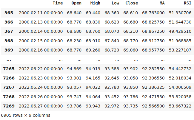
Fig 11: Training our model over 22 years of market data, excluding the period from 2023-2024.
Now let us label our data for machine learning. We want to help our model learn the changes in price given changes in our technical indicators. To help our model learn this relationship, we will transform our inputs to denote the current state of the indicator. For example, our RSI indicator will have 3 possible states:
- Above 70.
- Below 30.
- Between 70 and 30.
#MA States
data["MA 1"] = 0
data["MA 2"] = 0
data.loc[data["MA"] > data["MA"].shift(40),"MA 1"] = 1
data.loc[data["MA"] <= data["MA"].shift(40),"MA 2"] = 1

#RSI States
data["RSI 1"] = 0
data["RSI 2"] = 0
data["RSI 3"] = 0
data.loc[data["RSI"] < 30,"RSI 1"] = 1
data.loc[data["RSI"] > 70,"RSI 2"] = 1
data.loc[(data["RSI"] >= 30) & (data["RSI"] <= 70),"RSI 3"] = 1

#Target
data["Target"]    = data["Close"].shift(-22) - data["Close"]
data["MA Target"] = data["MA"].shift(-22) - data["MA"]

#Clean up the data
data = data.dropna()
data = data.iloc[40:,:]
data = data.reset_index(drop=True)
Now we can start measuring our accuracy.
from sklearn.linear_model import Ridge
from sklearn.model_selection import TimeSeriesSplit,cross_val_score
Applying these transformations, allows us to observe the average change in price as the RSI passes through the 3 zones we have specified. The coefficients of our linear model can be interpreted as the average change in price associated with each of the 3 RSI zones. These findings may sometimes go against classical teachings on how to use the indicator. For example, our Ridge model has learned that when the RSI reading surpasses 70, price levels tend to fall, otherwise when the RSI reading is less than 70, future price levels tend to rise.
#Our model can suggest optimal ways of using the RSI indicator
#Our model has learned that on average price tends to fall the RSI reading is less than 30 and increases otherwises
model = Ridge()

model.fit(data.loc[:,["RSI 1","RSI 2","RSI 3"]] , data["Target"])

model.coef_
Our Ridge model can predict future prices well only given the current state of the RSI.
#RSI state
np.mean(cross_val_score(Ridge(),data.loc[:,["RSI 1","RSI 2","RSI 3"]] , data["Target"],cv=tscv))
Likewise, our model has also learned its own trading rules from the changes in the moving average indicators. The first coefficient of the model is negative, meaning when the moving average rises over 40 candles, the moving average tends to fall. And the second coefficient is positive. Therefore, from the historical data we fetched in our Terminal, when the 40 period AUDJPY Daily moving average falls over 40 candles, they tend to rise afterward. Our model has learned a mean reverting strategy from the data.
#Our model can suggest optimal ways of using the RSI indicator
#Our model has learned that on average price tends to fall the RSI reading is less than 30 and increases otherwises
model = Ridge()

model.fit(data.loc[:,["MA 1","MA 2"]] , data["Target"])

model.coef_
Our model performs even better when we give it the current state of our moving average indicator.
#MA state
np.mean(cross_val_score(Ridge(),data.loc[:,["MA 1","MA 2"]] , data["Target"],cv=tscv))
Converting To ONNX
Now that we have found ideal input parameters for our Moving Average forecast, let us now prepare to convert our model to ONNX format. Open Neural Network Exchange (ONNX) allows us to build machine learning models in a language-agnostic framework. The ONNX protocol is an open-source initiative to create a universal standard representation for machine learning models, allowing us to build and deploy machine learning models in any language as long as it fully adopts the ONNX API.
First, let us fetch the data we need, according to the best inputs we have found.
#Fetch clean data
new_data = clean_data(140,130)
Import the libraries we need.
import onnx
from   skl2onnx import convert_sklearn
from   skl2onnx.common.data_types import FloatTensorType
Fit the RSI model on all the data we have.
#First we will export the RSI model
rsi_model = Ridge()
rsi_model.fit(data.loc[:,['RSI 1','RSI 2','RSI 3']],data.loc[:,'Target'])
Fit the moving average model on all the data we have.
#Finally we will export the MA model
ma_model = Ridge()
ma_model.fit(data.loc[:,['MA 1','MA 2']],data.loc[:,'MA Target'])
Define the input shape of our model and save it to the disk.
initial_types = [('float_input', FloatTensorType([1, 3]))]
onnx.save(convert_sklearn(rsi_model,initial_types=initial_types,target_opset=12),"AUDJPY D1 RSI AI F22 P40.onnx")

initial_types = [('float_input', FloatTensorType([1, 2]))]
onnx.save(convert_sklearn(ma_model,initial_types=initial_types,target_opset=12),"AUDJPY D1 MA AI F22 P40.onnx")
Implementing in MQL5
We are now ready to start building our trading application in MQL5. We want to build a trading application capable of entering and exiting its positions using our new-found insights on the moving averages. Not only that, we will generally guide our model using slower indicators that generate signals in a manner that is not too aggressive. Let us try and emulate how human traders are not always forcing a position on the market.
Additionally, we will also implement trailing stop losses to ensure sound risk management. We will use the Average True Range (ATR) indicator, to dynamically set our stop loss and take profit levels. Our strategy is based primarily on moving average channels.
Our strategy forecasts the moving averages 40 steps into the future to give us confirmation before we can open any position. We back tested this strategy over 1 year of historical data that was not shown to the model during training.
First, we will start by importing the ONNX file we have just created.
//+------------------------------------------------------------------+
//|                                                    GBPUSD AI.mq5 |
//|                                        Gamuchirai Zororo Ndawana |
//|                          https://www.mql5.com/en/gamuchiraindawa |
//+------------------------------------------------------------------+
#property copyright "Gamuchirai Zororo Ndawana"
#property link      "https://www.mql5.com/en/gamuchiraindawa"
#property version   "1.00"

//+------------------------------------------------------------------+
//| Load our resources                                               |
//+------------------------------------------------------------------+
#resource  "\\Files\\AUDJPY D1 MA AI F22 P40.onnx" as const uchar onnx_buffer[];
#resource  "\\Files\\AUDJPY D1 RSI AI F22 P40.onnx" as const uchar rsi_onnx_buffer[];
Then we will import the libraries we need.
//+------------------------------------------------------------------+
//| Libraries                                                        |
//+------------------------------------------------------------------+
#include <Trade\Trade.mqh>
CTrade Trade;
#include <Trade\OrderInfo.mqh>
class COrderInfo;
Now we shall define the global variables we need.
//+------------------------------------------------------------------+
//| Global variables                                                 |
//+------------------------------------------------------------------+
long     onnx_model;
int      ma_handler,state;
double   bid,ask,vol;
vectorf  model_forecast   = vectorf::Zeros(1);
vectorf  rsi_model_output = vectorf::Zeros(1);
double   min_volume,max_volume_increase, volume_step, buy_stop_loss, sell_stop_loss,atr_stop,risk_equity;
double   take_profit = 0;
double   close_price[3],atr_reading[],ma_buffer[];
long     min_distance,login;
int      atr,close_average,ticket_1,ticket_2;
bool     authorized = false;
double   margin,lot_step;
string   currency,server;
bool     all_closed =true;
int      rsi_handler;
long     rsi_onnx_model;
double   indicator_reading[];
ENUM_ACCOUNT_TRADE_MODE account_type;
const double  stop_percent = 1;
Let us define our input variables.
//+------------------------------------------------------------------+
//| Technical indicators                                             |
//+------------------------------------------------------------------+
input group "Money Management"
input int    lot_multiple     = 10; // How big should the lot size be?
input double profit_target = 0;     // Profit Target
input double loss_target   = 0;     // Max Loss Allowed

input group "Money Management"
const int    atr_period = 200;      //ATR Period
input double atr_multiple =2.5;     //ATR Multiple
Now we must define exactly how our trading application must be initialized. We will first check to ensure the user has given the application permission to trade. If we have permission to continue, then we will load our technical indicators and ONNX models.
int OnInit()
  {
//Authorization
   if(!TerminalInfoInteger(TERMINAL_TRADE_ALLOWED))
     {
      Comment("Press Ctrl + E To Give The Robot Permission To Trade And Reload The Program");
      return(INIT_FAILED);
     }

   else
      if(!MQLInfoInteger(MQL_TRADE_ALLOWED))
        {
         Comment("Reload The Program And Make Sure You Clicked Allow Algo Trading");
         return(INIT_FAILED);
        }

      else
        {
         Comment("This License is Genuine");
         setup();
        }
//Everything was okay
   return(INIT_SUCCEEDED);
  }
Whenever our trading application is no longer in use, we must free up the resources we are no longer using, to ensure our end user has a good experience with our application.
//+------------------------------------------------------------------+
//| Expert deinitialization function                                 |
//+------------------------------------------------------------------+
void OnDeinit(const int reason)
  {
   OnnxRelease(onnx_model);
   OnnxRelease(rsi_onnx_model);
   IndicatorRelease(atr)
  }
Whenever we receive updated price quotes, we shall update our variables and check for new trading opportunities. Otherwise, if we already have open trades, then let us update our trailing stop loss.
//+------------------------------------------------------------------+
//| Expert tick function                                             |
//+------------------------------------------------------------------+
void OnTick()
  {
//Update technical data
   update();

   if(PositionsTotal() == 0)
     {
      check_setup();
     }

   if(PositionsTotal() > 0)
     {
      check_atr_stop();
     }
  }
To get a prediction from our model, we have to define the current states of the RSI and moving average indicator.
//+------------------------------------------------------------------+
//| Get a prediction from our model                                  |
//+------------------------------------------------------------------+
int model_predict(void)
  {
//MA Forecast
   vectorf  model_inputs = vectorf::Zeros(2);
   vectorf  rsi_model_inputs = vectorf::Zeros(3);
   CopyBuffer(ma_handler,0,0,40,ma_buffer);

   if(ma_buffer[0] > ma_buffer[39])
     {
      model_inputs[0] = 1;
      model_inputs[1] = 0;
     }

   else
      if(ma_buffer[0] < ma_buffer[39])
        {
         model_inputs[1] = 1;
         model_inputs[0] = 0;
        }

//RSI Forecast
   CopyBuffer(rsi_handler,0,0,1,indicator_reading);

   if(indicator_reading[0] < 30)
     {
      rsi_model_inputs[0] = 1;
      rsi_model_inputs[1] = 0;
      rsi_model_inputs[2] = 0;
     }


   else
      if(indicator_reading[0] >70)
        {
         rsi_model_inputs[0] = 0;
         rsi_model_inputs[1] = 1;
         rsi_model_inputs[2] = 0;
        }

      else
        {
         rsi_model_inputs[0] = 0;
         rsi_model_inputs[1] = 0;
         rsi_model_inputs[2] = 1;
        }

//Model predictions
   OnnxRun(onnx_model,ONNX_DEFAULT,model_inputs,model_forecast);
   OnnxRun(rsi_onnx_model,ONNX_DEFAULT,rsi_model_inputs,rsi_model_output);


//Evaluate model output for buy setup
   if(((rsi_model_output[0] > 0)  && (model_forecast[0] > 0)))
     {
      //AI Models forecast
      Comment("AI Forecast: UP");
      return(1);
     }

//Evaluate model output for a sell setup
   if((rsi_model_output[0] < 0) && (model_forecast[0] < 0))
     {
      Comment("AI Forecast: DOWN");
      return(-1);
     }

//Otherwise no position was found
   return(0);
  }
Update our global variables. It is cleaner for us to perform these updates in one function call, as opposed to having all the code directly being executed in the OnTick() handler.
//+------------------------------------------------------------------+
//| Update our market data                                           |
//+------------------------------------------------------------------+
void update(void)
  {
   ask = SymbolInfoDouble(_Symbol,SYMBOL_ASK);
   bid = SymbolInfoDouble(_Symbol,SYMBOL_BID);
   buy_stop_loss = 0;
   sell_stop_loss = 0;
   static datetime time_stamp;
   datetime time = iTime(_Symbol,PERIOD_CURRENT,0);
   check_price(3);
   CopyBuffer(atr,0,0,1,atr_reading);
   CopyBuffer(ma_handler,0,0,1,ma_buffer);
   ArraySetAsSeries(atr_reading,true);
   atr_stop = ((min_volume + atr_reading[0]) * atr_multiple);
//On Every Candle
   if(time_stamp != time)
     {

      //Mark the candle
      time_stamp = time;
      OrderCalcMargin(ORDER_TYPE_BUY,_Symbol,min_volume,ask,margin);
     }
  }
Load the resources we need such as our technical indicators, account and market information and other data of that nature.
//+------------------------------------------------------------------+
//| Load resources                                                   |
//+------------------------------------------------------------------+
bool setup(void)
  {
//Account Info
   currency = AccountInfoString(ACCOUNT_CURRENCY);
   server = AccountInfoString(ACCOUNT_SERVER);
   login = AccountInfoInteger(ACCOUNT_LOGIN);

//Indicators
   atr = iATR(_Symbol,PERIOD_CURRENT,atr_period);

//Setup technical indicators
   ma_handler   =iMA(Symbol(),PERIOD_CURRENT,40,0,MODE_SMA,PRICE_LOW);
   vol          = SymbolInfoDouble(Symbol(),SYMBOL_VOLUME_MIN) * lot_multiple;
   rsi_handler  = iRSI(Symbol(),PERIOD_CURRENT,30,PRICE_CLOSE);

//Market Information
   min_volume = SymbolInfoDouble(_Symbol,SYMBOL_VOLUME_MIN);
   max_volume_increase = SymbolInfoDouble(_Symbol,SYMBOL_VOLUME_MAX) / SymbolInfoDouble(_Symbol,SYMBOL_VOLUME_MIN);
   min_distance = SymbolInfoInteger(_Symbol,SYMBOL_TRADE_STOPS_LEVEL);
   lot_step = SymbolInfoDouble(_Symbol,SYMBOL_VOLUME_STEP);

//Define our ONNX model
   ulong ma_input_shape [] = {1,2};
   ulong rsi_input_shape [] = {1,3};
   ulong output_shape [] = {1,1};

//Create the model
   onnx_model     = OnnxCreateFromBuffer(onnx_buffer,ONNX_DEFAULT);
   rsi_onnx_model = OnnxCreateFromBuffer(rsi_onnx_buffer,ONNX_DEFAULT);

   if((onnx_model == INVALID_HANDLE) || (rsi_onnx_model == INVALID_HANDLE))
     {
      Comment("[ERROR] Failed to load AI module correctly");
      return(false);
     }

//Validate I/O
   if((!OnnxSetInputShape(onnx_model,0,ma_input_shape)) || (!OnnxSetInputShape(rsi_onnx_model,0,rsi_input_shape)))
     {
      Comment("[ERROR] Failed to set input shape correctly: ",GetLastError());
      return(false);
     }

   if((!OnnxSetOutputShape(onnx_model,0,output_shape)) || (!OnnxSetOutputShape(rsi_onnx_model,0,output_shape)))
     {
      Comment("[ERROR] Failed to load AI module correctly: ",GetLastError());
      return(false);
     }
//Everything went fine
   return(true);
  }
Putting it all together, this is what our trading application looks like.
//+------------------------------------------------------------------+
//|                                                    GBPUSD AI.mq5 |
//|                                        Gamuchirai Zororo Ndawana |
//|                          https://www.mql5.com/en/gamuchiraindawa |
//+------------------------------------------------------------------+
#property copyright "Gamuchirai Zororo Ndawana"
#property link      "https://www.mql5.com/en/gamuchiraindawa"
#property version   "1.00"

//+------------------------------------------------------------------+
//| Load our resources                                               |
//+------------------------------------------------------------------+
#resource  "\\Files\\AUDJPY D1 MA AI F22 P40.onnx" as const uchar onnx_buffer[];
#resource  "\\Files\\AUDJPY D1 RSI AI F22 P40.onnx" as const uchar rsi_onnx_buffer[];

//+------------------------------------------------------------------+
//| Libraries                                                        |
//+------------------------------------------------------------------+
#include <Trade\Trade.mqh>
CTrade Trade;
#include <Trade\OrderInfo.mqh>
class COrderInfo;

//+------------------------------------------------------------------+
//| Global variables                                                 |
//+------------------------------------------------------------------+
long     onnx_model;
int      ma_handler,state;
double   bid,ask,vol;
vectorf  model_forecast   = vectorf::Zeros(1);
vectorf  rsi_model_output = vectorf::Zeros(1);
double   min_volume,max_volume_increase, volume_step, buy_stop_loss, sell_stop_loss,atr_stop,risk_equity;
double   take_profit = 0;
double   close_price[3],atr_reading[],ma_buffer[];
long     min_distance,login;
int      atr,close_average,ticket_1,ticket_2;
bool     authorized = false;
double   margin,lot_step;
string   currency,server;
bool     all_closed =true;
int      rsi_handler;
long     rsi_onnx_model;
double   indicator_reading[];
ENUM_ACCOUNT_TRADE_MODE account_type;
const double  stop_percent = 1;

//+------------------------------------------------------------------+
//| Technical indicators                                             |
//+------------------------------------------------------------------+
input group "Money Management"
input int    lot_multiple     = 10; // How big should the lot size be?
input double profit_target = 0;     // Profit Target
input double loss_target   = 0;     // Max Loss Allowed

input group "Money Management"
input int    bb_period = 36;        //Bollinger band period
input int    ma_period = 4;         //Moving average period
const int    atr_period = 200;      //ATR Period
input double atr_multiple =2.5;      //ATR Multiple

//+------------------------------------------------------------------+
//| Expert initialization function                                   |
//+------------------------------------------------------------------+
int OnInit()
  {
//Authorization
   if(!TerminalInfoInteger(TERMINAL_TRADE_ALLOWED))
     {
      Comment("Press Ctrl + E To Give The Robot Permission To Trade And Reload The Program");
      return(INIT_FAILED);
     }

   else
      if(!MQLInfoInteger(MQL_TRADE_ALLOWED))
        {
         Comment("Reload The Program And Make Sure You Clicked Allow Algo Trading");
         return(INIT_FAILED);
        }

      else
        {
         Comment("This License is Genuine");
         setup();
        }
//--- Everything was okay
   return(INIT_SUCCEEDED);
  }
//+------------------------------------------------------------------+
//| Expert deinitialization function                                 |
//+------------------------------------------------------------------+
void OnDeinit(const int reason)
  {
//---
   OnnxRelease(onnx_model);
   OnnxRelease(rsi_onnx_model);
  }
//+------------------------------------------------------------------+
//| Expert tick function                                             |
//+------------------------------------------------------------------+
void OnTick()
  {
//--- Update technical data
   update();

   if(PositionsTotal() == 0)
     {
      check_setup();
     }

   if(PositionsTotal() > 0)
     {
      check_atr_stop();
     }
  }
//+------------------------------------------------------------------+
//| Get a prediction from our model                                  |
//+------------------------------------------------------------------+
int model_predict(void)
  {
//MA Forecast
   vectorf  model_inputs = vectorf::Zeros(2);
   vectorf  rsi_model_inputs = vectorf::Zeros(3);
   CopyBuffer(ma_handler,0,0,40,ma_buffer);

   if(ma_buffer[0] > ma_buffer[39])
     {
      model_inputs[0] = 1;
      model_inputs[1] = 0;
     }

   else
      if(ma_buffer[0] < ma_buffer[39])
        {
         model_inputs[1] = 1;
         model_inputs[0] = 0;
        }

//RSI Forecast
   CopyBuffer(rsi_handler,0,0,1,indicator_reading);

   if(indicator_reading[0] < 30)
     {
      rsi_model_inputs[0] = 1;
      rsi_model_inputs[1] = 0;
      rsi_model_inputs[2] = 0;
     }


   else
      if(indicator_reading[0] >70)
        {
         rsi_model_inputs[0] = 0;
         rsi_model_inputs[1] = 1;
         rsi_model_inputs[2] = 0;
        }

      else
        {
         rsi_model_inputs[0] = 0;
         rsi_model_inputs[1] = 0;
         rsi_model_inputs[2] = 1;
        }

//Model predictions
   OnnxRun(onnx_model,ONNX_DEFAULT,model_inputs,model_forecast);
   OnnxRun(rsi_onnx_model,ONNX_DEFAULT,rsi_model_inputs,rsi_model_output);


//Evaluate model output for buy setup
   if(((rsi_model_output[0] > 0)  && (model_forecast[0] > 0)))
     {
      //AI Models forecast
      Comment("AI Forecast: UP");
      return(1);
     }

//Evaluate model output for a sell setup
   if((rsi_model_output[0] < 0) && (model_forecast[0] < 0))
     {
      Comment("AI Forecast: DOWN");
      return(-1);
     }

//Otherwise no position was found
   return(0);
  }

//+------------------------------------------------------------------+
//| Check for valid trade setups                                     |
//+------------------------------------------------------------------+
void check_setup(void)
  {
   int res = model_predict();

   if(res == -1)
     {
      Trade.Sell(vol,Symbol(),bid,0,0,"VD V75 AI");
      state = -1;
     }

   else
      if(res == 1)
        {
         Trade.Buy(vol,Symbol(),ask,0,0,"VD V75 AI");
         state = 1;
        }
  }

//+------------------------------------------------------------------+
//| Update our market data                                           |
//+------------------------------------------------------------------+
void update(void)
  {
   ask = SymbolInfoDouble(_Symbol,SYMBOL_ASK);
   bid = SymbolInfoDouble(_Symbol,SYMBOL_BID);
   buy_stop_loss = 0;
   sell_stop_loss = 0;
   static datetime time_stamp;
   datetime time = iTime(_Symbol,PERIOD_CURRENT,0);
   check_price(3);
   CopyBuffer(atr,0,0,1,atr_reading);
   CopyBuffer(ma_handler,0,0,1,ma_buffer);
   ArraySetAsSeries(atr_reading,true);
   atr_stop = ((min_volume + atr_reading[0]) * atr_multiple);
//On Every Candle
   if(time_stamp != time)
     {

      //Mark the candle
      time_stamp = time;
      OrderCalcMargin(ORDER_TYPE_BUY,_Symbol,min_volume,ask,margin);
     }
  }

//+------------------------------------------------------------------+

//+------------------------------------------------------------------+
//| Load resources                                                   |
//+------------------------------------------------------------------+
bool setup(void)
  {
//Account Info
   currency = AccountInfoString(ACCOUNT_CURRENCY);
   server = AccountInfoString(ACCOUNT_SERVER);
   login = AccountInfoInteger(ACCOUNT_LOGIN);

//Indicators
   atr = iATR(_Symbol,PERIOD_CURRENT,atr_period);

//Setup technical indicators
   ma_handler   =iMA(Symbol(),PERIOD_CURRENT,40,0,MODE_SMA,PRICE_LOW);
   vol          = SymbolInfoDouble(Symbol(),SYMBOL_VOLUME_MIN) * lot_multiple;
   rsi_handler  = iRSI(Symbol(),PERIOD_CURRENT,30,PRICE_CLOSE);

//Market Information
   min_volume = SymbolInfoDouble(_Symbol,SYMBOL_VOLUME_MIN);
   max_volume_increase = SymbolInfoDouble(_Symbol,SYMBOL_VOLUME_MAX) / SymbolInfoDouble(_Symbol,SYMBOL_VOLUME_MIN);
   min_distance = SymbolInfoInteger(_Symbol,SYMBOL_TRADE_STOPS_LEVEL);
   lot_step = SymbolInfoDouble(_Symbol,SYMBOL_VOLUME_STEP);

//Define our ONNX model
   ulong ma_input_shape [] = {1,2};
   ulong rsi_input_shape [] = {1,3};
   ulong output_shape [] = {1,1};

//Create the model
   onnx_model     = OnnxCreateFromBuffer(onnx_buffer,ONNX_DEFAULT);
   rsi_onnx_model = OnnxCreateFromBuffer(rsi_onnx_buffer,ONNX_DEFAULT);

   if((onnx_model == INVALID_HANDLE) || (rsi_onnx_model == INVALID_HANDLE))
     {
      Comment("[ERROR] Failed to load AI module correctly");
      return(false);
     }

//--- Validate I/O
   if((!OnnxSetInputShape(onnx_model,0,ma_input_shape)) || (!OnnxSetInputShape(rsi_onnx_model,0,rsi_input_shape)))
     {
      Comment("[ERROR] Failed to set input shape correctly: ",GetLastError());
      return(false);
     }

   if((!OnnxSetOutputShape(onnx_model,0,output_shape)) || (!OnnxSetOutputShape(rsi_onnx_model,0,output_shape)))
     {
      Comment("[ERROR] Failed to load AI module correctly: ",GetLastError());
      return(false);
     }
//--- Everything went fine
   return(true);
  }

//+------------------------------------------------------------------+
//| Close all our open positions                                     |
//+------------------------------------------------------------------+
void close_all()
  {
   if(PositionsTotal() > 0)
     {
      ulong ticket;
      for(int i =0;i < PositionsTotal();i++)
        {
         ticket = PositionGetTicket(i);
         Trade.PositionClose(ticket);
        }
     }
  }

//+------------------------------------------------------------------+
//| Update our trailing ATR stop                                     |
//+------------------------------------------------------------------+
void check_atr_stop()
  {

   for(int i = PositionsTotal() -1; i >= 0; i--)
     {

      string symbol = PositionGetSymbol(i);
      if(_Symbol == symbol)
        {

         ulong ticket = PositionGetInteger(POSITION_TICKET);
         double position_price = PositionGetDouble(POSITION_PRICE_OPEN);
         double type = PositionGetInteger(POSITION_TYPE);
         double current_stop_loss = PositionGetDouble(POSITION_SL);

         if(type == POSITION_TYPE_BUY)
           {
            double atr_stop_loss = (ask - (atr_stop));
            double atr_take_profit = (ask + (atr_stop));

            if((current_stop_loss < atr_stop_loss) || (current_stop_loss == 0))
              {
               Trade.PositionModify(ticket,atr_stop_loss,atr_take_profit);
              }
           }

         else
            if(type == POSITION_TYPE_SELL)
              {
               double atr_stop_loss = (bid + (atr_stop));
               double atr_take_profit = (bid - (atr_stop));
               if((current_stop_loss > atr_stop_loss) || (current_stop_loss == 0))
                 {
                  Trade.PositionModify(ticket,atr_stop_loss,atr_take_profit);
                 }
              }
        }
     }
  }

//+------------------------------------------------------------------+
//| Close our open buy positions                                     |
//+------------------------------------------------------------------+
void close_buy()
  {
   ulong ticket;
   int type;
   if(PositionsTotal() > 0)
     {
      for(int i = 0; i < PositionsTotal();i++)
        {
         if(PositionGetSymbol(i) == _Symbol)
           {
            ticket = PositionGetTicket(i);
            type = (int)PositionGetInteger(POSITION_TYPE);
            if(type == POSITION_TYPE_BUY)
              {
               Trade.PositionClose(ticket);
              }
           }
        }
     }
  }

//+------------------------------------------------------------------+
//| Close our open sell positions                                    |
//+------------------------------------------------------------------+
void close_sell()
  {
   ulong ticket;
   int type;
   if(PositionsTotal() > 0)
     {
      for(int i = 0; i < PositionsTotal();i++)
        {
         if(PositionGetSymbol(i) == _Symbol)
           {
            ticket = PositionGetTicket(i);
            type = (int)PositionGetInteger(POSITION_TYPE);
            if(type == POSITION_TYPE_SELL)
              {
               Trade.PositionClose(ticket);
              }
           }
        }
     }
  }

//+------------------------------------------------------------------+
//| Get the most recent price values                                 |
//+------------------------------------------------------------------+
void check_price(int candles)
  {
   for(int i = 0; i < candles;i++)
     {
      close_price[i] = iClose(_Symbol,PERIOD_CURRENT,i);
     }
  }
//+------------------------------------------------------------------+
Let us now back test our trading algorithm using data we did not show the algorithm when we were training it. The period we have selected runs from the beginning of January 2023 until June 28, 2024, on Daily market quotes on the AUDJPY Pair. We will set the "Forward" parameter to "No" because we have made sure the dates we selected were not observed when we trained the model.
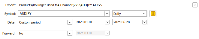
Fig 12: The Symbol and Time Frame we will use to evaluate our trading strategy.
Additionally, we will mimic real trading conditions by first setting the "Delays" parameter to "Random delay". This parameter controls the latency between when our orders are placed and when they get executed. Setting it to be random, is similar to what real life trading is like, our latency is not constant at all times. Furthermore, we will instruct our Terminal to model the market using real ticks. This setting will slow down our back test slightly because the terminal will first have to fetch detailed market data from our broker over the internet.
The last parameters, controlling the account deposit and leverage, should be adjusted to suit your trading setup. Assuming we successfully fetch all the data we requested, our back test will begin.
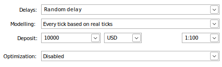
Fig 13:The parameters which we will use for our back test.
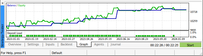
Fig 14: The performance of our strategy on data our model was not trained on.
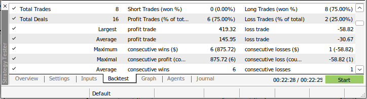
Fig 12: More details of our back test on unseen market data.
Conclusion
The broad market data we have analyzed today is clearly telling us that if you wish to forecast intervals less than 40 steps into the future, you may probably be better off predicting price directly. However, if you desire to forecast more than 40 steps into the future, may most likely be better off predicting the change in the moving average as opposed to the change in price. There are always more enhancements waiting for us to observe them and the difference they make. We can clearly see that any amount of time spent transforming the inputs of the data is worth it because it allows us to expose the underlying relationships to our models in a more meaningful way
Warning: All rights to these materials are reserved by MetaQuotes Ltd. Copying or reprinting of these materials in whole or in part is prohibited.
This article was written by a user of the site and reflects their personal views. MetaQuotes Ltd is not responsible for the accuracy of the information presented, nor for any consequences resulting from the use of the solutions, strategies or recommendations described.

- Free trading apps
- Over 8,000 signals for copying
- Economic news for exploring financial markets
You agree to website policy and terms of use
The result shown looks promising; will try this out.
More of this kind please.
Thanks.
The article Trait Engineering with Python and MQL5 (Part I) has been published: AI models for long-term forecasting on moving averages:
Author: Gamuchirai Zororo Ndawana
Some of the pictures are not showing...
The results look promising.
More stuff like this please.
More stuff like this please. thank you.
You're welcome Too Che Ng.
There is definitely still a lot more that can be said given such a strong start.
Some images are not displayed...
I'm sorry to hear that, I'm sure moderators will get around to fixing that, given they already have a lot to do as things stand.