Self Optimizing Expert Advisor With MQL5 And Python (Part VI): Taking Advantage of Deep Double Descent

Overfitting in machine learning can take on many different forms. Most commonly, it happens when an AI model learns too much of the noise in the data, and fails to make any useful generalizations. This leads to dismal performance when we assess the model on data it has not seen before. There are many techniques that have been developed to mitigate overfitting, but such methods can often prove challenging to implement, especially when you are just getting started on your journey. However, a recent paper, published by a group of diligent Harvard Alumni, suggests that on certain tasks, overfitting may be a problem of the past. This article will walk you through the research paper, and demonstrate how you can build world-class AI models, inline with the world's leading research.

Overview Of The Methodology

There are many techniques used to detect overfitting when developing AI models. The most trusted method, is to examine the plots of the test and training error of the model. Initially, the two plots may drop together, which is a good sign. As we continue training our model, we will hit an optimal error level, and once we go past that, our training error continues to fall, but our test error only gets worse. Many techniques have been developed to remedy this problem, such as early stopping. Early stopping, terminates the training procedure, if the model's validation error doesn't significantly change, or continually deteriorates. Afterward, the best weights are restored, and it is assumed the best model has been located, as in Fig 1 below.

Fig 1: A generalized plot demonstrating over fitting in practice

These ideas have been shaken to their very foundations by a 2019 research paper titled "Deep Double Descent", the link is provided here. The paper does not attempt to explain the phenomenon it demonstrates, it only describes the characteristics of the phenomenon that had been observed at the time of writing.  In essence, the paper demonstrates that on certain problems, the test error of the model will fall at first, before it begins to rise and then dramatically fall a second time, to new lows before the model finally converges, as demonstrated in Fig 2 below.

Fig 2: Visualizing the deep double descent phenomenon

The paper demonstrates that this phenomenon can be conceptualized as a function of:

1. The parameters in the model.
2. The maximum number of training iterations.

This is to say, if you continually trained larger and larger models on the same dataset, we will observe that our test error will first fall before it starts rising, and if we continue training larger models, we will observe our test error drop a second time, to new lows, creating an error plot similar to Fig 2 above. However, progressively training larger and larger models isn't always feasible due to the computational cost. For our discussion, we will explore the deep double descent phenomenon as a function of the maximum number of iterations we allow.

The idea is that, as we allow our model to perform more training iterations, its validation error will always increase, before it drops to new lows. The amount of time taken for the model to hit its peak error levels and start falling varies, depending on various factors, such as the amount of noise in the dataset and the type of model being trained.

There are no widely accepted explanations for the phenomenon, but so far, the easiest way to grasp the phenomenon is when we imagine double descent as a function of the model's parameters.

Imagine we start with a simple neural network, the model will most likely under fit our data. Meaning, its performance could improve by adding more complexity to the model. As we increase the complexity of our neural network, we slowly approach a point whereby our model fits our data exactly.  In traditional machine learning, we are taught that the model's training error will always fall if we make our model more complex. This is true. However, it is not the complete truth.

Once our model is complex enough to fit our data perfectly, at this point the training error is typically a quantity very close to 0, and it stops falling as we make our model more complex. This is the first blow to the traditional ideologies of machine learning. This point in commonly referred to as the interpolation threshold. If we continue increasing the model's complexity past this threshold, we will observe a remarkable drop in test accuracy. And in most cases, the model's error rates will fall to new lows and stabilize there.

Algorithms meant to mitigate over-fitting, such as early stopping, appear to have been unintentionally holding us back. These algorithms will always terminate the training procedure before we will observe the second descent. Let us recreate the double descent phenomenon, to independently observe it for ourselves.

Getting Started

We will first need to extract our data from our MetaTrader 5 platform using a script we built in MQL5.

//+------------------------------------------------------------------+
//|                                                      ProjectName |
//|                                      Copyright 2020, CompanyName |
//|                                       http://www.companyname.net |
//+------------------------------------------------------------------+
#property copyright "Gamuchirai Zororo Ndawana"
#property link      "https://www.mql5.com/en/users/gamuchiraindawa"
#property version   "1.00"
#property script_show_inputs

//+------------------------------------------------------------------+
//| Script Inputs                                                    |
//+------------------------------------------------------------------+
input int size = 100000; //How much data should we fetch?

//+------------------------------------------------------------------+
//| Global variables                                                 |
//+------------------------------------------------------------------+

//+------------------------------------------------------------------+
//| On start function                                                |
//+------------------------------------------------------------------+
void OnStart()
  {

//--- File name
   string file_name = "Market Data " + Symbol()+  ".csv";

//--- Write to file
   int file_handle=FileOpen(file_name,FILE_WRITE|FILE_ANSI|FILE_CSV,",");

   for(int i= size;i>=0;i--)
     {
      if(i == size)
        {
         FileWrite(file_handle,"Time","Open","High","Low","Close");
        }

      else
        {
         FileWrite(file_handle,iTime(Symbol(),PERIOD_CURRENT,i),
                   iOpen(Symbol(),PERIOD_CURRENT,i),
                   iHigh(Symbol(),PERIOD_CURRENT,i),
                   iLow(Symbol(),PERIOD_CURRENT,i),
                   iClose(Symbol(),PERIOD_CURRENT,i)
                  );
        }
     }
//--- Close the file
   FileClose(file_handle);
  }
//+------------------------------------------------------------------+

To get started, let us first import the libraries we need.

#Standard libraries
import pandas                  as     pd
import numpy                   as     np
import seaborn                 as     sns
import matplotlib.pyplot       as     plt
from   mpl_toolkits.mplot3d    import Axes3D
from   sklearn.linear_model    import LinearRegression
from   sklearn.neural_network  import MLPRegressor
from   sklearn.metrics         import mean_squared_error
from   sklearn.model_selection import cross_val_score,TimeSeriesSplit

Now, read in the data.

#Read in the data
data = pd.read_csv('GBPUSD_Daily_20160103_20240131.csv',sep='\t')

Let us clean up our data.

#Clean up the data
data.rename(columns={'<OPEN>':'Open','<HIGH>':'High','<LOW>':'Low','<CLOSE>':'Close'},inplace=True)

Drop the unnecessary columns.

#Drop columns we don't need
data = data.drop(['<DATE>','<VOL>','<SPREAD>','<TICKVOL>'],axis=1)
data

Visualizing the data.

#Plot the close price
plt.plot(data["Close"])
plt.xlabel("Time")
plt.ylabel("Close Price")
plt.title("GBPUSD Daily Close")

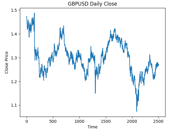
Fig 3: The GBPUSD Daily OHLC data we will be working with

We want to train a model that forecasts the Daily returns of the GBPUSD. However, there are 2 variables we have to choose:

1. At what frequency should we calculate the returns?
2. How far into the future should we forecast?

Typically, we forecast 1 step into the future, and we calculate the returns as the difference between 2 consecutive days. However, is this truly optimal? Is this the best we can do at all times? We will not answer this question, the data itself will answer this question for us.

Let us perform a grid search for the parameters for our returns and our forecast horizon. First, we need to define a uniform axis for both parameters.

#Define the input range
x_min , x_max = 2,100 #Look ahead
y_min , y_max = 2,100 #Period

Now, define the x and y-axis.

#Sample input range uniformly
x_axis = np.arange(x_min,x_max,4) #Look ahead
y_axis = np.arange(y_min,y_max,4) #Period

We need to create a mesh-grid. The mesh-grid is 2 individual, 2-dimensional arrays, that can be used together to map all possible input combinations we want to evaluate.

#Create a meshgrid
x , y = np.meshgrid(x_axis,y_axis)

This function will be used to clean up the data-set before we test our model's accuracy with the new settings we would like to evaluate.

#This function will create and return a clean dataframe according to our specifications
def clean_data(look_ahead,period):
    #Create a copy of the data
    temp = pd.read_csv('GBPUSD_Daily_20160103_20240131.csv',sep='\t')
    #Clean up the data
    temp.rename(columns={'<OPEN>':'Open','<HIGH>':'High','<LOW>':'Low','<CLOSE>':'Close'},inplace=True)
    temp = temp.drop(['<DATE>','<VOL>','<SPREAD>','<TICKVOL>'],axis=1)
    #Define our target
    temp["Target"] = temp["Close"].shift(-look_ahead)
    #Apply the differencing
    temp["Close"] = temp["Close"].diff(period)
    temp["Open"] = temp["Open"].diff(period)
    temp["High"] = temp["High"].diff(period)
    temp["Low"] = temp["Low"].diff(period)
    temp = temp.dropna()
    temp = temp.reset_index(drop=True)
    return(temp)

Our next function, will cross-validate our model under the settings we pass, and return its cross validation error.

#Evaluate the objective function
def evaluate(look_ahead,period):
    #Define the model
    model = LinearRegression()
    #Define our time series split
    tscv = TimeSeriesSplit(n_splits=5,gap=look_ahead)
    temp = clean_data(look_ahead,period)
    score = np.mean(cross_val_score(model,temp.loc[:,["Open","High","Low","Close"]],temp["Target"],cv=tscv))
    return(score)

Finally, we need a function that will record our results in an array that has the same shape as either one of our mesh-grids.

#Define the objective
def objective(x,y):
    #Define the output matrix
    results = np.zeros([x.shape[0],y.shape[0]])
    #Fill in the output matrix
    for i in np.arange(0,x.shape[0]):
        #Select the rows
        look_ahead = x[i]
        period     = y[i]
        for j in np.arange(0,y.shape[0]):
            results[i,j] = evaluate(look_ahead[j],period[j])
    return(results)

So far, we have implemented the functions we need to see how our model's error levels change as we change the interval with which we calculate our returns and how far into the future we wish to forecast. Let us first observe how a simple model behaves as we change these parameters, before we start dealing with more complex, deep neural networks.

linear_reg_res = objective(x,y)
linear_reg_res = np.abs(linear_reg_res)

A contour plot is commonly used in geography to show changes in altitudes over a terrain. We can use these surface plots, to find which pair of parameters produce the lowest error levels from our simple linear regression model. The blue regions, are combinations that produced low error, while the red regions are unsatisfactory combinations. The white dot, in the darkest blue region of our contour plot, represents the best forecasting settings for our linear regression model.

As we can see from the plot below, our simple linear AI model would have easily outperformed any trader in the market that was using the classical return period of 1 and forecasting 1 step into the future.

plt.contourf(x,y,linear_reg_res,100,cmap="jet")
plt.plot(x_axis[linear_reg_res.min(axis=0).argmin()],y_axis[linear_reg_res.min(axis=1).argmin()],'.',color='white')
plt.ylabel("Differencing Period")
plt.xlabel("Forecast Horizon")
plt.title("Linear Regression Accuracy Forecasting GBPUSD Daily Close")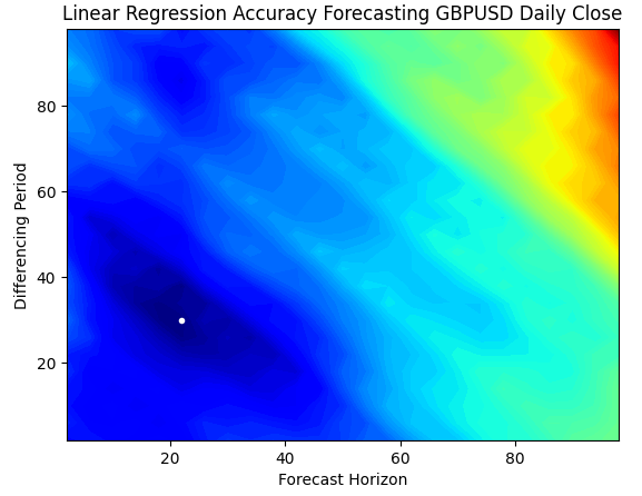

Fig 4: Our contour plot of our linear regression's accuracy forecasting the GBPUSD Daily

Visualizing the results in 3D generates a surface, that allows us to visualize our model's relationship with the GBPUSD market. The plot shows us that as we forecast further into the future our error rates drop, to an optimal level, and start to increase as we keep looking further forward into the future. However, the most important take away is that for our linear model, Fig 5 below clearly shows that our best model inputs are in the 20 to 40 range for both our forecast horizon and returns period.

#Create a surface plot
fig , ax = plt.subplots(subplot_kw={"projection":"3d"})
fig.set_size_inches(8,8)
ax.plot_surface(x,y,linear_reg_res,cmap="jet")

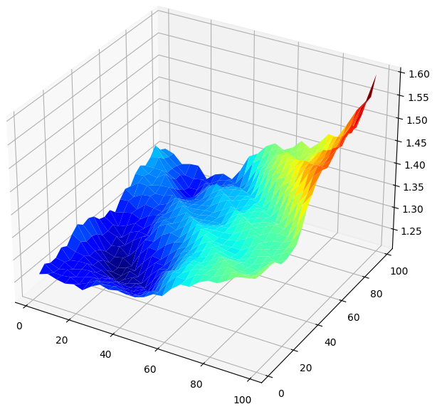
Fig 5: Visualizing our Linear model's error forecasting the GBPUSD Daily returns

Now that we are familiar with contour and surface plots, let us observe how our deep neural network performs, when we use it to search over the same parameter space.

res = objective(x,y)
res = np.abs(res)

Our neural networks surface plot is exponentially more complex to visualize. The blue zones are desirable because they represent combinations that produced low error levels. However, notice that we observe red zones abruptly appearing in the middle of optimal combinations. This is quite interesting, isn't it?

How can 2 combinations be so close together, and yet have vastly different error levels? This is partly due to the nature of the optimization algorithms used to train neural networks. If we were to train this model a second time, we would obtain a different plot entirely, with a different optimal point.

plt.contourf(x,y,res,100,cmap="jet")
plt.plot(x_axis[res.min(axis=0).argmin()],y_axis[res.min(axis=1).argmin()],'.',color='white')
plt.ylabel("Differencing Period")
plt.xlabel("Forecast Horizon")
plt.title("Neural Network Accuracy Forecasting GBPUSD Daily Close")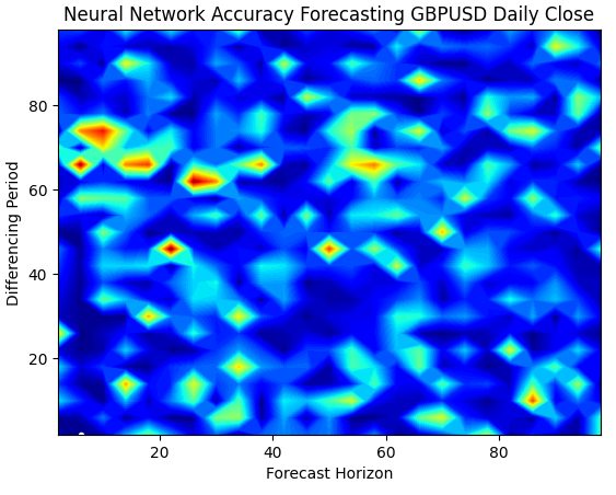

Fig 6: Neural networks are very sensitive to the inputs we have

When we visualize the model's performance in 3D, we can see how unstable neural networks can be. Can we confidently say that the neural network has effectively learned any useful relationships? Which model is performing better so far? If we approach the problem from the traditional school of thought, we will select the simple linear model because it is creating smoother error plots, which may be a sign it has more skill and the volatile error rates of the neural network could be seen as a sign it's overfitting the data.

However, that is a classical approach to machine learning, from the contemporary school of thought, we see the error plots of the neural network as an indication that the model has not yet truly converged, not as an indication it is overfitting. In other words, according to the Double Descent paper, it is still too early for us to compare the neural network. Let us try and independently prove this to ourselves, instead of blindly trusting research papers due to the accreditation of the authors.

#Create a surface plot
fig , ax = plt.subplots(subplot_kw={"projection":"3d"})
fig.set_size_inches(8,8)
ax.plot_surface(x,y,res,cmap="jet")

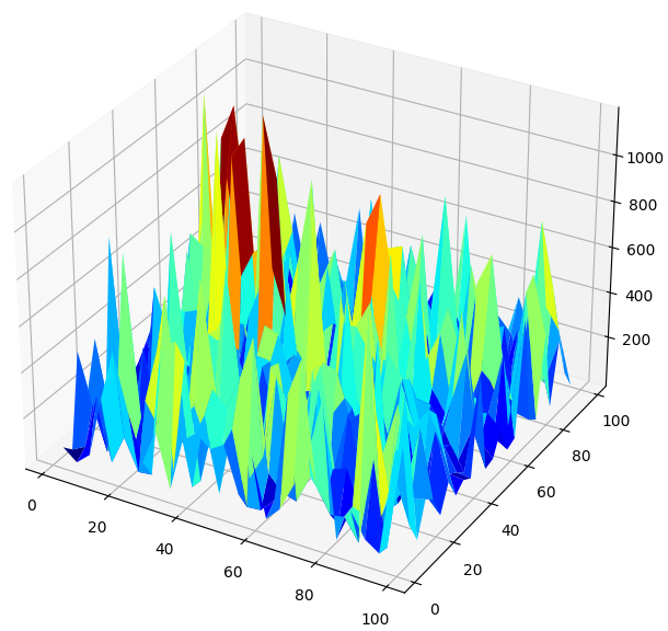
Fig 7: Our neural networks error levels forecasting the GBPUSD Daily return

Checking For Double Descent

We will first apply the best parameters we have found for calculating the returns and how far into the future we should be forecasting.

#The best settings we have found so far
look_ahead = x_axis[res.min(axis=0).argmin()]
difference_period = y_axis[res.min(axis=1).argmin()]
data["Target"] = data["Close"].shift(-look_ahead)
#Apply the differencing
data["Close"] = data["Close"].diff(difference_period)
data["Open"] = data["Open"].diff(difference_period)
data["High"] = data["High"].diff(difference_period)
data["Low"] = data["Low"].diff(difference_period)
data.dropna(inplace=True)
data.reset_index(drop=True,inplace=True)
data

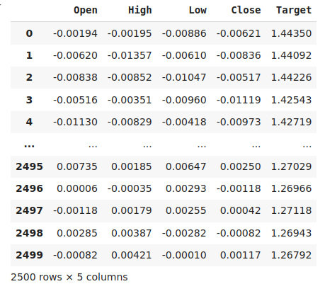
Fig 8: Our data in its current form

Importing the libraries we need.

from sklearn.model_selection import train_test_split,TimeSeriesSplit
from sklearn.metrics         import mean_squared_error

Define the maximum number of epochs. Recall that double descent is a function of the model complexity or the maximum number of training iterations. We will test this with a simple neural network and vary the maximum number of iterations. Our maximum number of training iterations with be progressive powers of 2.

max_epoch = 50

Creating a data-frame to store our error levels.

err_rates = pd.DataFrame(columns = np.arange(0,max_epoch),index=["Train","Validation","Test"])

We need to set our time series split object.

tscv = TimeSeriesSplit(n_splits=5,gap=look_ahead)

Now perform a train test split.

train , test = train_test_split(data,shuffle=False,test_size=0.5)

Cross validating our model as we increase the maximum number of iterations as uniform powers of 2.

for j in np.arange(0,max_epoch):
  #Define our model and measure its error
  current_train_err = []
  current_val_err = []
  model = MLPRegressor(hidden_layer_sizes=(6,5),max_iter=(2 ** j))

  for i,(train_index,test_index) in enumerate(tscv.split(train)):
    #Assess the model
    model.fit(train.loc[train_index,["Open","High","Low","Close"]],train.loc[train_index,'Target'])
    current_train_err.append(mean_squared_error(train.loc[train_index,'Target'],model.predict(train.loc[train_index,["Open","High","Low","Close"]])))
    current_val_err.append(mean_squared_error(train.loc[test_index,'Target'],model.predict(train.loc[test_index,["Open","High","Low","Close"]])))

  #Record our observations
  err_rates.loc["Train",j]      = np.mean(current_train_err)
  err_rates.loc["Validation",j] = np.mean(current_val_err)
  err_rates.loc["Test",j]       = mean_squared_error(test['Target'],model.predict(test.loc[:,["Open","High","Low","Close"]]))

Our first 6 iterations show how our models error rates changed as we went from 1 to 32 training iterations. As we can see from the plot below, our test error started by dropping, then started increasing, before making a higher low. Our training and validation error rates started by increasing before dropping to a slightly higher low, and increasing again. However, 32 iterations only represent a small interval of the training procedure, let's observe how the rest of the training procedure unfolds.

plt.plot(err_rates.iloc[0,0:5])
plt.plot(err_rates.iloc[1,0:5])
plt.plot(err_rates.iloc[2,0:5])
plt.legend(["Train Error","Validation Error","Test Error"])
plt.ylabel("RMSE")
plt.xlabel("Epochs: Our Epochs Are Indices of 2")
plt.title("Neural Network Accuracy Forecasting GBPUSD Daily Close")

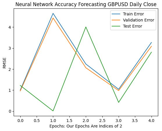
Fig 9: Our validation accuracy as we go from 1 to 32 iterations

As we move on, we now see how our model's error rates evolve over the 64 to 256 interval. It appears that after some divergence, our error rates are finally converging to a minimum. However, according to the paper, we have a long way to go.

Let the reader note, by default scikit-learn instantiates neural networks that perform only 200 iterations. This is a number slightly smaller than 2 to the power 8. And with algorithms such as early stopping, we would've been trapped in deceptive local optima, somewhere in the hills and troughs of the uneven surface we observed in Fig 7 above 

plt.plot(err_rates.iloc[0,0:9])
plt.plot(err_rates.iloc[1,0:9])
plt.plot(err_rates.iloc[2,0:9])
plt.legend(["Train Error","Validation Error","Test Error"])
plt.ylabel("RMSE")
plt.xlabel("Epochs: Our Epochs Are Indices of 2")
plt.title("Neural Network Accuracy Forecasting GBPUSD Daily Close")

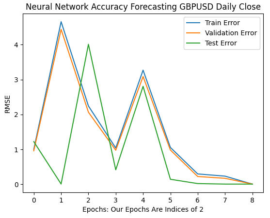
Fig 10: Our model's error rates are starting to converge

Our optimal error rates were produced when our model was allowed to perform more than 1 billion iterations! The exact number is 2 to the power 30. This point is marked by the red vertical line in Fig 11 below. We normally perform fractions of the optimal number of iterations, out of fear of overfitting the data, leaving us trapped us in suboptimal error levels to the left of the red line.

plt.plot(err_rates.iloc[0,:])
plt.plot(err_rates.iloc[1,:])
plt.plot(err_rates.iloc[2,:])
plt.axvline(err_rates.loc["Test",:].argmin(),color='red')
plt.legend(["Train Error","Validation Error","Test Error","Double Descent Error"])
plt.ylabel("RMSE")
plt.xlabel("Epochs: Our Epochs Are Indices of 2")
plt.title("Neural Network Accuracy Forecasting GBPUSD Daily Close")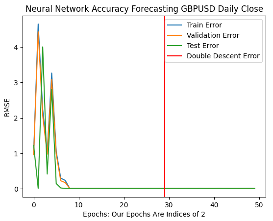

Fig 11: Our double descent error levels are marked by the red vertical line, and to the left we can observe the classical domain of traditional machine learning

Optimizing Our Neural Network

Clearly, there some merit in the paper. Under normal circumstances, we would not even remotely consider allowing numerous iterations, out of fear of overfitting. We can now confidently optimize our model without the fear of overfitting to the training data.

from sklearn.model_selection import RandomizedSearchCV

Initialize the model.

#Reinitialize the model
model = MLPRegressor(max_iter=(err_rates.loc["Test",:].argmin()))

Let us define the parameters we want to search over.

#Define the tuner
tuner = RandomizedSearchCV(
        model,
        {
        "activation" : ["relu","logistic","tanh","identity"],
        "solver":["adam","sgd","lbfgs"],
        "alpha":[0.1,0.01,0.001,0.0001,0.00001,0.00001,0.0000001],
        "tol":[0.1,0.01,0.001,0.0001,0.00001,0.000001,0.0000001],
        "learning_rate":['constant','adaptive','invscaling'],
        "learning_rate_init":[0.1,0.01,0.001,0.0001,0.00001,0.000001,0.0000001],
        "hidden_layer_sizes":[(1,4),(5,8,10),(5,10,20),(10,50,10),(20,5),(1,5),(20,10)],
        "early_stopping":[True,False],
        "warm_start":[True,False],
        "shuffle": [True,False]
        },
        n_iter=2**9,
        cv=5,
        n_jobs=-1,
        scoring="neg_mean_squared_error"
)

Finally, fit the tuner object.

tuner.fit(train.loc[:,["Open","High","Low","Close"]],train.loc[:,"Target"])

The best parameters we found.

tuner.best_params_

{'warm_start': True,
 'tol': 0.1,
 'solver': 'lbfgs',
 'shuffle': False,
 'learning_rate_init': 1e-06,
 'learning_rate': 'adaptive',
 'hidden_layer_sizes': (5, 8, 10),
 'early_stopping': False,
 'alpha': 1e-05,
 'activation': 'relu'}

Converting To ONNX

Now that we have created our model, we can convert it to ONNX format. ONNX stands for Open Neural Network Exchange, and it is an open-source protocol that allows us to create and deploy AI models in any programming language that extends support to the ONNX API specification. MQL5 allows us to import our AI models and deploy them directly into our terminals. First, we will import the libraries we need.

import onnx
from skl2onnx import convert_sklearn
from skl2onnx.common.data_types import FloatTensorType

Then, let us fit our model on all the data we have.

model = tuner.best_estimator_.fit(train.loc[:,["Open","High","Low","Close"]],train.loc[:,"Target"])

Specify the input shape of your model.

#Define the input shape of 1,4
initial_type = [('float_input', FloatTensorType([1, 4]))]
#Specify the input shape
onnx_model = convert_sklearn(model, initial_types=initial_type)

Save the ONNX model.

#Save the onnx model
onnx.save(onnx_model,"GBPUSD DAILY.onnx")

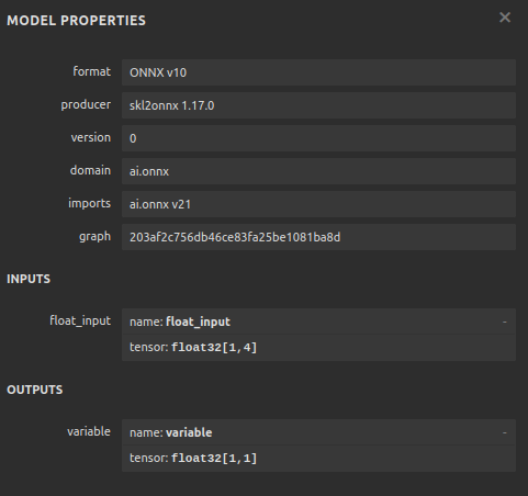
Fig 12: Our ONNX model's input and output parameters

 

Implementation in MQL5

We can now get started implementing our trading strategy in MQL5. Our strategy will be based on the Daily time-frame. We will use a combination of the Bollinger Bands and Moving averages to determine the prevailing market trend.

The Bollinger Bands are commonly used to identify securities that are overbought or oversold. Commonly, when price levels reach the upper band, the security under observation is considered overbought. Typically, it when price levels are overbought, traders expect future price levels to fall and revert to the average price level. We will instead use the Bollinger Band in a trend following fashion.

When price levels cross above the mid-line of the Bands, we will consider that a strong bullish signal, and the opposite is true when price levels fall beneath the middle band, we will take that as a strong sell signal. Such simple trading rules are bound to generate too many signals, which may not always be ideal. We will instead filter price fluctuations by considering moving average values instead of price action itself.

We will apply 2 moving averages, one on the high price and the other on the low price, to create a moving average channel. Our entries signals will be generated when both moving averages cross the Bollinger Band mid-line, and our AI signal forecasts that price will indeed move in that direction. 

Finally, our positions will be closed whenever the moving average channels cross the Bollinger Band mid-line, or if the moving average channel falls back within the Bollinger Bands after breaking out of the Bands, whichever will occur first.

Let us get started by first loading our ONNX model.

//+------------------------------------------------------------------+
//|                                                    GBPUSD AI.mq5 |
//|                                        Gamuchirai Zororo Ndawana |
//|                          https://www.mql5.com/en/gamuchiraindawa |
//+------------------------------------------------------------------+
#property copyright "Gamuchirai Zororo Ndawana"
#property link      "https://www.mql5.com/en/gamuchiraindawa"
#property version   "1.00"

//+------------------------------------------------------------------+
//| Load our ONNX file                                               |
//+------------------------------------------------------------------+
#resource  "\\Files\\GBPUSD DAILY.onnx" as const uchar onnx_buffer[];

Next, we need to load the Trade library for help managing our positions.

//+------------------------------------------------------------------+
//| Libraries                                                        |
//+------------------------------------------------------------------+
#include <Trade\Trade.mqh>
CTrade Trade;

We also need a few global variables for data we will share in different parts of our application.

//+------------------------------------------------------------------+
//| Global variables                                                 |
//+------------------------------------------------------------------+
bool   patience = true;
long   onnx_model;
int    bb_handler,ma_h_handler,ma_l_handler;
double ma_h_buffer[],ma_l_buffer[];
double bb_h_buffer[],bb_m_buffer[],bb_l_buffer[];
int    state;
double bid,ask;
vectorf model_forecast = vectorf::Zeros(1);

Our technical indicators have period parameters we want our end user to be able to adjust as market conditions change.

//+------------------------------------------------------------------+
//| User Inputs                                                      |
//+------------------------------------------------------------------+
input group "Technical Indicators"
input int bb_period = 60;
input int ma_period = 14;

The first time our application is loaded, we will first load our technical indicators before loading our ONNX model. We will use the ONNX buffer we defined at the beginning of our program to create an ONNX model from that buffer. From there, we will validate that our ONNX model is sound and that our input and output parameters are inline with our specifications.

//+------------------------------------------------------------------+
//| Expert initialization function                                   |
//+------------------------------------------------------------------+
int OnInit()
  {
//--- Setup technical indicators
   bb_handler   = iBands(Symbol(),PERIOD_D1,bb_period,0,1,PRICE_CLOSE);
   ma_h_handler = iMA(Symbol(),PERIOD_D1,ma_period,0,MODE_SMA,PRICE_HIGH);
   ma_l_handler = iMA(Symbol(),PERIOD_D1,ma_period,0,MODE_SMA,PRICE_LOW);
//--- Define our ONNX model
   ulong input_shape [] = {1,4};
   ulong output_shape [] = {1,1};
//--- Create the model
   onnx_model = OnnxCreateFromBuffer(onnx_buffer,ONNX_DEFAULT);

   if(onnx_model == INVALID_HANDLE)
     {
      Comment("[ERROR] Failed to load AI module correctly");
      return(INIT_FAILED);
     }

//--- Validate I/O
   if(!OnnxSetInputShape(onnx_model,0,input_shape))
     {
      Comment("[ERROR] Failed to set input shape correctly: ",GetLastError()," Actual shape: ",OnnxGetInputCount(onnx_model));
      return(INIT_FAILED);
     }

   if(!OnnxSetOutputShape(onnx_model,0,output_shape))
     {
      Comment("[ERROR] Failed to load AI module correctly: ",GetLastError()," Actual shape: ",OnnxGetOutputCount(onnx_model));
      return(INIT_FAILED);
     }


//--- Everything was okay
   return(INIT_SUCCEEDED);
  }

If our trading application is no longer in use, we will release the resources we are no longer using.

//+------------------------------------------------------------------+
//| Expert deinitialization function                                 |
//+------------------------------------------------------------------+
void OnDeinit(const int reason)
  {
//---
   OnnxRelease(onnx_model);
   IndicatorRelease(bb_handler);
   IndicatorRelease(ma_h_handler);
   IndicatorRelease(ma_l_handler);
  }

Finally, whenever we receive new price quotes, we shall update our global variables. From there, our next step to take, depends on the number of positions we have open. If none, we will search for an entry signal. Otherwise, we will check for exit signals.

//+------------------------------------------------------------------+
//| Expert tick function                                             |
//+------------------------------------------------------------------+
void OnTick()
  {
//--- Update technical data
   update();

   if(PositionsTotal() == 0)
     {
      patience = true;
      check_setup();
     }

   if(PositionsTotal() > 0)
     {
      string direction = model_forecast[0] > iClose(Symbol(),PERIOD_D1,0) ? "UP" : "DOWN";
      Comment("Model Forecast: ",model_forecast[0]," ",direction);
      close_setup();
     }
  }

The following function will get a forecast from our model.

//+------------------------------------------------------------------+
//| Get a prediction from our model                                  |
//+------------------------------------------------------------------+
void model_predict(void)
  {
   double o,h,l,c;
   vector op,hi,lo,cl;
   op.CopyRates(Symbol(),PERIOD_D1,COPY_RATES_OPEN,0,3);
   hi.CopyRates(Symbol(),PERIOD_D1,COPY_RATES_HIGH,0,3);
   lo.CopyRates(Symbol(),PERIOD_D1,COPY_RATES_LOW,0,3);
   cl.CopyRates(Symbol(),PERIOD_D1,COPY_RATES_CLOSE,0,3);

   o =  op[2]  - op[0];
   h =  hi[2]  - hi[0];
   l =  lo[2]  - lo[0];
   c =  cl[2]  - cl[0];

   vectorf model_inputs = vectorf::Zeros(4);
   model_inputs[0] = o;
   model_inputs[1] = h;
   model_inputs[2] = l;
   model_inputs[3] = c;

   OnnxRun(onnx_model,ONNX_DEFAULT,model_inputs,model_forecast);
  }

Now we will define how our application should close its positions. The patience boolean is used to control when the application should close our positions. If the moving average channel has not broken out of the Bollinger Bands when our positions were initially opened, the patience variable will be set to true. The value will remain true, until the moving average channel breaks out of the Bands. At that point, the patience flag is set to false, and if the channel falls back within the bands, our positions will be closed.

//+------------------------------------------------------------------+
//| Close our open positions                                         |
//+------------------------------------------------------------------+
void close_setup(void)
  {
   if(patience)
     {
      if(state == 1)
        {
         if(ma_l_buffer[0] > bb_h_buffer[0])
           {
            patience = false;
           }


         if((ma_h_buffer[0] < bb_m_buffer[0]) && (ma_l_buffer[0] < bb_m_buffer[0]))
           {
            Trade.PositionClose(Symbol());
           }
        }

      else
         if(state == -1)
           {
            if(ma_h_buffer[0] < bb_l_buffer[0])
              {
               patience = false;
              }

            if((ma_h_buffer[0] > bb_m_buffer[0]) && (ma_l_buffer[0] > bb_m_buffer[0]))
              {
               Trade.PositionClose(Symbol());
              }
           }
     }

   else
     {
      if((state == -1) && (ma_l_buffer[0] > bb_l_buffer[0]))
        {
         Trade.PositionClose(Symbol());
        }

      if((state == 1) && (ma_h_buffer[0] < bb_h_buffer[0]))
        {
         Trade.PositionClose(Symbol());
        }
     }

  }

For us to consider the setup valid, we want the moving average channel to be completely on one side of the mid-band and our AI forecast to agree with the price action. Otherwise, we will simply wait instead of chasing fleeting fluctuations in price.

//+------------------------------------------------------------------+
//| Check for valid trade setups                                     |
//+------------------------------------------------------------------+
void check_setup(void)
  {

   if((ma_h_buffer[0] < bb_m_buffer[0]) && (ma_l_buffer[0] < bb_m_buffer[0]))
     {
      model_predict();
      if((model_forecast[0] < iClose(Symbol(),PERIOD_CURRENT,0)))
        {
         if(ma_h_buffer[0] < bb_l_buffer[0])
            patience = false;

         Trade.Sell(0.3,Symbol(),bid,0,0,"GBPUSD AI");
         state = -1;
        }
     }

   if((ma_h_buffer[0] > bb_m_buffer[0]) && (ma_l_buffer[0] > bb_m_buffer[0]))
     {
      model_predict();
      if(model_forecast[0] > iClose(Symbol(),PERIOD_CURRENT,0))
        {
         if(ma_l_buffer[0] > bb_h_buffer[0])
            patience = false;

         Trade.Buy(0.3,Symbol(),ask,0,0,"GBPUSD AI");
         state = 1;
        }
     }
  }

Finally, we need a function responsible for updating our global variables.

//+------------------------------------------------------------------+
//| Update our market data                                           |
//+------------------------------------------------------------------+
void update(void)
  {
   CopyBuffer(bb_handler,0,0,1,bb_m_buffer);
   CopyBuffer(bb_handler,1,0,1,bb_h_buffer);
   CopyBuffer(bb_handler,2,0,1,bb_l_buffer);
   CopyBuffer(ma_h_handler,0,0,1,ma_h_buffer);
   CopyBuffer(ma_l_handler,0,0,1,ma_l_buffer);
  }
//+------------------------------------------------------------------+

We can now back test our trading strategy. We used the strategy tester to evaluate our application over roughly 3 years of GBPUSD Daily market data. Note that when we built our AI model, we used Daily market data from 2016 until 2024. Therefore, the back test we have shown below, is effectively testing our AI strategy on data the model has already seen. Note that, even though our model has been exposed to the data and trained well, our account balance was very volatile over time.

This demonstrates that although we have trained our model well, AI models do not  "remember" what they "learned" in the sense a human does. It tries to create a formula that generalizes well to the data. Meaning it may still make mistakes on data it was already trained on.

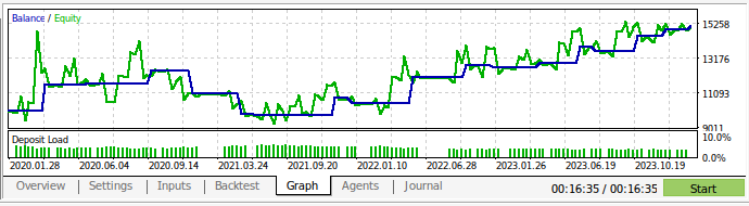
Fig 13: We back tested our application over roughly 3 years of Daily GBPUSD market data

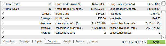
Fig 14: Our model's trading performance details

Conclusion

To recap, we have demonstrated that the appearance of "overfitting" may in some circumstances only be a call for greater effort. The classical ideology of overfitting AI models, has to a certain extent, kept us stuck in suboptimal error levels. However, we are confident that after reading this article, you will be able to make better use of your models. Let the reader recall that we also had the option of simply increasing the number of hidden layers in the model, or simply training a model with one layer, and increase the width of the model's layer. However, training such massive models will require an entirely different approach, requiring skills in parallel computing.

This article has furnished you with a computationally inexpensive approach of training a basic model of a fixed size instead and using Daily Data due to the small number of rows we will have to process on such a time frame. However, for our results to be conclusive and robust, we may need to instead reduce our training set to half its size so that our model is trained from 2016 to 2020 and all the data from 2020 to 2024 is not exposed to our model during training.