
Neural Networks Made Easy (Part 90): Frequency Interpolation of Time Series (FITS)

Introduction
Time series analysis plays an important role in making management decisions in financial markets. Time series data in finance is often complex and dynamic, and its processing requires efficient methods.
Sophisticated models and methods are developed within the advanced research in time series analysis. However, these models are often computationally intensive, making them less suitable for use in dynamic financial market conditions. That is, they can hardly be applied when the timing of a decision is crucial.
In addition, nowadays more and more management decisions are made using mobile devices, which are also limited in resources. This fact places additional demands on the models used in making such decisions.
In this context, representing time series in the frequency domain can provide a more efficient and compact representation of the observed patterns. For example, spectral data and high amplitude frequency analysis can help identify important features.
In the previous articles, we discussed the FEDformer method that uses the frequency domain to find patterns in a time series. However, the Transformer used in that method can hardly be referred to as a lightweight model. Instead of complex models that require large computational costs, the paper "FITS: Modeling Time Series with 10k Parameters" proposes a method for the frequency interpolation of time series (Frequency Interpolation Time Series - FITS). It is a compact and efficient solution for time series analysis and forecasting. FITS uses frequency domain interpolation to expand the window of the analyzed time segment, thus enabling the efficient extraction of temporal features without significant computational overhead.
The authors of the FITS method highlight the following advantages of their method:
- FITS is a lightweight model with a small number of parameters, making it an ideal choice for use on devices with limited resources.
- FITS uses a complex neural network to collect information about the amplitude and phase of the signal, which improves the efficiency of time series data analysis.
1. FITS Algorithm
Time series analysis in the frequency domain allows the signal to be decomposed into a linear combination of sinusoidal components without data loss. Each of these components has a unique frequency, initial phase, and amplitude. While forecasting a time series can be a challenging task, forecasting individual sinusoidal components is relatively simpler since it only requires adjusting the phase of the sine wave based on the time shift. The sinusoidal waves shifted in this way are linearly combined to obtain predicted values of the analyzed time series.
This approach allows us to effectively preserve the frequency characteristics of the analyzed time series window. It also maintains the semantic sequence between the time window and the forecast horizon.
However, predicting each sinusoidal component in the time domain can be quite labor-intensive. To solve this problem, the authors of the FITS method propose the use of a complex frequency domain, which provides a more compact and informative data representation.
Fast Fourier Transform (FFT) efficiently transforms discrete time series signals from the time domain to the complex frequency domain. In Fourier analysis, the complex frequency domain is represented by a sequence in which each frequency component is characterized by a complex number. This complex number reflects the amplitude and phase of the component, providing a complete description. The amplitude of a frequency component represents the magnitude, or strength, of that component in the original signal in the time domain. In contrast, phase indicates the time shift or delay introduced by that component. Mathematically, a complex number associated with a frequency component can be represented as a complex exponential element with a given amplitude and phase:
![]()
where X(f) is a complex number associated with a frequency component at frequency f,
|X(f)| is the amplitude of the component,
θ(f) is the phase of the component.
In the complex plane, the exponential element can be represented as a vector with a length equal to the amplitude and an angle equal to the phase:
![]()
Thus, a complex number in the frequency domain provides a concise and elegant way to represent the amplitude and phase of each frequency component in the Fourier transform.
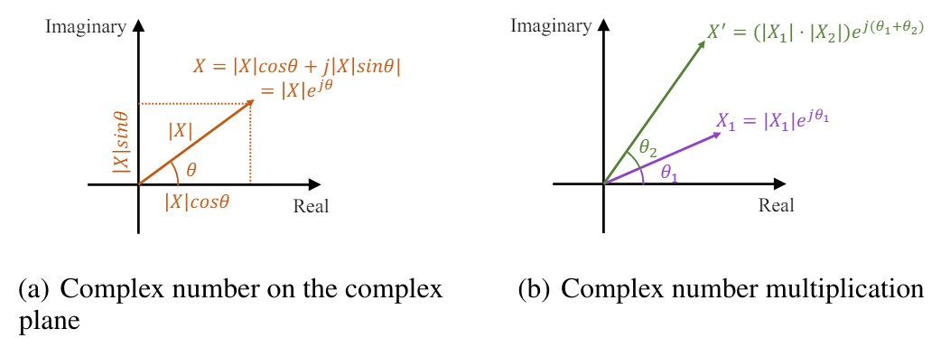
The time shift of a signal corresponds to the phase shift in the frequency domain. In the domain of complex frequencies, such a phase shift can be expressed as the multiplication of a unit element of a complex exponential by the corresponding phase. The shifted signal still has an amplitude of |X(f)|, and the phase shows a linear shift in time.
Thus, the amplitude scaling and phase shift can be simultaneously expressed as multiplication of complex numbers.
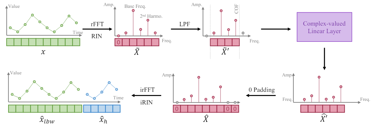
Based on fact that a longer time series provides a higher frequency resolution in its frequency representation, the authors of the FITS method train the model to expand a time series segment by interpolating the frequency representation of the analyzed window of the input data. They propose using a single complex linear layer to train such interpolation. As a result, the model can learn the amplitude scaling and phase shift as a multiplication of complex numbers during the interpolation process. In the FITS algorithm, the fast Fourier transform is used to project time series segments into the complex frequency domain. After interpolation, the frequency representation is projected back into the time representation using the inverse FFT.
However, the mean of such segments will result in a very large zero-frequency component in its complex frequency representation. To solve this problem, the received signal is passed through reversible normalization (RevIN), which allows us to obtain an instance with zero mean.
In addition, the authors of the method supplement FITS with a low pass filter (LPF) to reduce the size of the model. The low-pass filter effectively removes high-frequency components above a specified cutoff frequency, compacting the model representation while preserving important time series information.
Despite operating in the frequency domain, FITS is trained in the time domain using standard loss functions such as Mean Squared Error (MSE) after inverse fast Fourier transform. This provides a versatile approach that can be adapted to a variety of subsequent time series problems.
In forecasting tasks, FITS generates a retrospective analysis window together with the planning horizon. This enables control over forecasting and retrospective analysis, with the model being encouraged to accurately reconstruct the retrospective analysis window. The analysis conducted in the cited paper shows that a combination of hindsight and forecast monitoring can lead to improved performance in certain scenarios.
For reconstruction tasks, FITS subsamples the input time series segment based on a specified subsampling rate. Then it performs frequency interpolation, which allows the downsampled segment to be restored back to its original form. Thus, direct control using losses is applied to ensure accurate signal reconstruction.
To control the length of the model result tensor, the authors of the method introduce an interpolation rate, denoted as 𝜂, which is the ratio of the required size of the model result tensor to the corresponding size of the original data tensor.
It is noteworthy that when applying a low-pass filter (LPF), the size of the input data tensor of our complex layer corresponds to the cutoff frequency (COF) of LPF. After performing frequency interpolation, the complex frequency representation is padded with zeros to the required size of the result tensor. Before applying the reverse FFT, the introduce an additional zero as a component of the zero frequency representation.
The main purpose of inclusion of the LPF into FITS is to compress the model volume while preserving important information. LPF achieves this by discarding frequency components above a given cutoff frequency (COF), resulting in a more concise frequency domain representation. LPF preserves relevant information in the time series while discarding components that are beyond the model's learning capabilities. This ensures that a significant portion of the meaningful content of the input time series is preserved. Experiments conducted by the authors of the method show that the filtered signal exhibits minimal distortion even when only a quarter of the original representation in the frequency domain is preserved. Moreover, the high frequency components filtered with LPF typically contain noise that is inherently irrelevant for effective time series modeling.
The difficult task here is to select a suitable cutoff frequency (COF). To solve this problem, the authors of FITS propose a method based on the harmonic content of the dominant frequency. Harmonics, which are integer multiples of the dominant frequency, play an important role in shaping the waveform of a time series signal. By comparing the cutoff frequency with these harmonics, we preserve the corresponding frequency components associated with the structure and periodicity of the signal. This approach exploits the inherent relationship between frequencies to extract meaningful information while suppressing noise and unnecessary high-frequency components.
The original author's visualization of the FITS method is presented below.
2. Implementing in MQL5
We have considered the theoretical aspects of the FITS method. Now we can move to the practical implementation of the proposed approaches using MQL5.
As usual, we will use the proposed approaches, but our implementation will differ from the author's vision of the algorithm due to the specifics of the problem we are solving.
2.1 FFT implementation
From the theoretical description of the method presented above, it can be seen that it is based on direct and inverse fast Fourier decomposition. Using the fast Fourier decomposition, we first translate the analyzed signal into the frequency domain, and then return the predicted sequence to the time series representation. In this case, we can see two main advantages of the fast Fourier transform:
- Speed of operations compared to other similar transformations
- The ability to express the inverse transformation through the direct one
It should be noted here that within the framework of our task, we need the implementation of FFT of multivariate time series. In practice, it is the FFT applied to each unitary time series in our multivariate sequence.
Most mathematical operations in our implementations are transferred to OpenCL. This allows us to distribute the execution of a large number of similar operations with independent data across several parallel threads. This reduces the time required to execute operations. So, we will perform fast Fourier decomposition operations on the OpenCL side. In each of the parallel threads, we will perform decomposition of a separate unitary time series.
We will formalize the algorithm for performing operations in the form of an FFT kernel. In the kernel parameters, we will pass pointers to 4 data arrays. Here we use two arrays for the input data and the results of the operations. One array contains the real part of the complex value (the signal amplitude), and the second contains the imaginary part (its phase).
However, please note that we will not always feed the imaginary part of the signal to the kernel. For example, when decomposing the input time series, we don't have this part. In this situation, the solution is quite simple: we will replace the missing data with zero values. In order not to pass a separate buffer filled with zero values, we will create an input_complex flag in the kernel parameters.
The second point to note is that the Cooley-Tukey algorithm we use for FFT only works for sequences whose length is a power of 2. This condition imposes serious restrictions. However, this restriction concerns the preparation of the analyzed signal. The method works fine if we fill the missing elements of the sequence with zero values. Again, to avoid unnecessary copying of data to reformat the time series, we will add two variables to the kernel parameters: input_window and output_window. In the first variable, we indicate the actual length of the sequence under analysis, and in the second one, we indicate the size of the decomposition result vector, which is a power of 2. In this case we are talking about the sizes of a unitary sequence.
One more parameter, reverse, indicates the direction of the operation: direct or inverse transformation.
__kernel void FFT(__global float *inputs_re,
                  __global float *inputs_im,
                  __global float *outputs_re,
                  __global float *outputs_im,
                  const int input_window,
                  const int input_complex,
                  const int output_window,
                  const int reverse
                 )
  {
   size_t variable = get_global_id(0);
In the kernel body, we first define a thread identifier that will point us to the unitary sequence being analyzed. Here we will also define shifts in data buffers and other necessary constants.
   const ulong N = output_window;
   const ulong N2 = N / 2;
   const ulong inp_shift = input_window * variable;
   const ulong out_shift = output_window * variable;
In the next step, we re-sort the input data in a specific order, which will allow us to optimize the FFT algorithm a little.
   uint target = 0;
   for(uint position = 0; position < N; position++)
     {
      if(target > position)
        {
         outputs_re[out_shift + position] = (target < input_window ? inputs_re[inp_shift + target] : 0);
         outputs_im[out_shift + position] = ((target < input_window && input_complex) ?
                                                                     inputs_im[inp_shift + target] : 0);
         outputs_re[out_shift + target] = inputs_re[inp_shift + position];
         outputs_im[out_shift + target] = (input_complex ? inputs_im[inp_shift + position] : 0);
        }
      else
        {
         outputs_re[out_shift + position] = inputs_re[inp_shift + position];
         outputs_im[out_shift + position] = (input_complex ? inputs_im[inp_shift + position] : 0);
        }
      unsigned int mask = N;
      while(target & (mask >>= 1))
         target &= ~mask;
      target |= mask;
     }
Next comes the direct transformation of data, which is performed in a system of nested cycles. In the outer loop, we build FFT iterations for segments of length 2, 4, 8, ... n.
  float real = 0, imag = 0;
   for(int len = 2; len <= (int)N; len <<= 1)
     {
      float w_real = (float)cos(2 * M_PI_F / len);
      float w_imag = (float)sin(2 * M_PI_F / len);
In the body of the loop, we define a multiplier for the argument rotation per 1 point of the loop length and organize a nested loop for iterating over the blocks in the sequence being analyzed.
      for(int i = 0; i < (int)N; i += len)
        {
         float cur_w_real = 1;
         float cur_w_imag = 0;
Here we declare the variables of the current phase rotation and organize another nested loop over the elements in the block.
         for(int j = 0; j < len / 2; j++)
           {
            real = cur_w_real * outputs_re[out_shift + i + j + len / 2] -
                   cur_w_imag * outputs_im[out_shift + i + j + len / 2];
            imag = cur_w_imag * outputs_re[out_shift + i + j + len / 2] +
                   cur_w_real * outputs_im[out_shift + i + j + len / 2];
            outputs_re[out_shift + i + j + len / 2] = outputs_re[out_shift + i + j] - real;
            outputs_im[out_shift + i + j + len / 2] = outputs_im[out_shift + i + j] - imag;
            outputs_re[out_shift + i + j] += real;
            outputs_im[out_shift + i + j] += imag;
            real = cur_w_real * w_real - cur_w_imag * w_imag;
            cur_w_imag = cur_w_imag * w_real + cur_w_real * w_imag;
            cur_w_real = real;
           }
        }
     }
In the loop body, we first modify the elements being analyzed, and then change the value of the current phase variables for the next iteration.
Please note that modification of buffer elements is performed "in place" without allocating additional memory.
After the loop system iterations are complete, we check the value of the reverse flag. If we perform the reverse transformation, we will re-sort the data in the result buffer. In this case, we divide the obtained values by the number of elements in the sequence.
   if(reverse)
     {
      outputs_re[0] /= N;
      outputs_im[0] /= N;
      outputs_re[N2] /= N;
      outputs_im[N2] /= N;
      for(int i = 1; i < N2; i++)
        {
         real = outputs_re[i] / N;
         imag = outputs_im[i] / N;
         outputs_re[i] = outputs_re[N - i] / N;
         outputs_im[i] = outputs_im[N - i] / N;
         outputs_re[N - i] = real;
         outputs_im[N - i] = imag;
        }
     }
  }
2.2 Combining the real and imaginary parts of the predicted distribution
The kernel presented above allows performing direct and inverse fast Fourier decomposition, which quite covers our needs. But there is one more point in the FITS method, which should be paid attention to. The authors of the method use a complex neural network to interpolate data. For a detailed introduction to complex neural networks, I suggest you read the article "A Survey of Complex-Valued Neural Networks". In this implementation, we will use existing classes of neural layers that will separately interpolate the real and imaginary parts and then combine them according to the following formula:
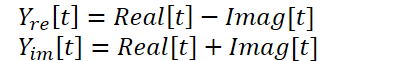
To perform these operations, we will create the ComplexLayer kernel. The kernel algorithm is quite simple. We just identify a thread in two dimensions that points to a row and a column of matrices. We determine shifts in data buffers and perform simple mathematical operations.
__kernel void ComplexLayer(__global float *inputs_re,
                           __global float *inputs_im,
                           __global float *outputs_re,
                           __global float *outputs_im
                          )
  {
   size_t i = get_global_id(0);
   size_t j = get_global_id(1);
   size_t total_i = get_global_size(0);
   size_t total_j = get_global_size(1);
   uint shift = i * total_j + j;
//---
   outputs_re[shift] = inputs_re[shift] - inputs_im[shift];
   outputs_im[shift] = inputs_im[shift] + inputs_re[shift];
  }
The ComplexLayerGradient backpropagation kernel is constructed in a similar way. You can study this code using the attached files.
This concludes our operations on the OpenCL program side.
2.3 Creating a FITS Method Class
After finishing working with the OpenCL program kernels, we move on to the main program, where we will create the CNeuronFITSOCL class to implement the approaches proposed by the FITS method authors. The new class will be derived from the neural layer base class CNeuronBaseOCL. The structure of the new class is shown below.
class CNeuronFITSOCL :  public CNeuronBaseOCL
  {
protected:
   //---
   uint              iWindow;
   uint              iWindowOut;
   uint              iCount;
   uint              iFFTin;
   uint              iIFFTin;
   //---
   CNeuronBaseOCL    cInputsRe;
   CNeuronBaseOCL    cInputsIm;
   CNeuronBaseOCL    cFFTRe;
   CNeuronBaseOCL    cFFTIm;
   CNeuronDropoutOCL cDropRe;
   CNeuronDropoutOCL cDropIm;
   CNeuronConvOCL    cInsideRe1;
   CNeuronConvOCL    cInsideIm1;
   CNeuronConvOCL    cInsideRe2;
   CNeuronConvOCL    cInsideIm2;
   CNeuronBaseOCL    cComplexRe;
   CNeuronBaseOCL    cComplexIm;
   CNeuronBaseOCL    cIFFTRe;
   CNeuronBaseOCL    cIFFTIm;
   CBufferFloat      cClear;
   //---
   virtual bool      FFT(CBufferFloat *inp_re, CBufferFloat *inp_im, CBufferFloat *out_re, CBufferFloat *out_im,
                                                                                           bool reverse = false);
   virtual bool      ComplexLayerOut(CBufferFloat *inp_re, CBufferFloat *inp_im,
                                     CBufferFloat *out_re, CBufferFloat *out_im);
   virtual bool      ComplexLayerGradient(CBufferFloat *inp_re, CBufferFloat *inp_im,
                                          CBufferFloat *out_re, CBufferFloat *out_im);
   //---
   virtual bool      feedForward(CNeuronBaseOCL *NeuronOCL);
   virtual bool      updateInputWeights(CNeuronBaseOCL *NeuronOCL);
   virtual bool      calcInputGradients(CNeuronBaseOCL *NeuronOCL);

public:
                     CNeuronFITSOCL(void) {};
                    ~CNeuronFITSOCL(void) {};
   //---
   virtual bool      Init(uint numOutputs, uint myIndex, COpenCLMy *open_cl,
                          uint window, uint window_out, uint count, float dropout,
                          ENUM_OPTIMIZATION optimization_type, uint batch);
   //---
   virtual bool      Save(int const file_handle);
   virtual bool      Load(int const file_handle);
   //---
   virtual int       Type(void)        const                      {  return defNeuronFITSOCL; }
   virtual void      SetOpenCL(COpenCLMy *obj);
   virtual void      TrainMode(bool flag);
   //---
   virtual bool      WeightsUpdate(CNeuronBaseOCL *source, float tau);
  };
The structure of the new class contains quite a lot of declarations of internal neural layer objects. This seems strange considering the expected simplicity of the model. However, please note that we will only train the parameters of 4 nested neural layers responsible for data interpolation (cInsideRe* and cInsideIm*). Other objects act as intermediate data buffers. We will consider their purpose while implementing the methods.
Also, pay attention that we have two CNeuronDropoutOCL layers. In this implementation, I will not use LFP, which involves determining a certain cutoff frequency. Here I remembered the experiments of the authors of the FEDformer method who speak about the efficiency of sampling a set of frequency characteristics. So I decided to use a Dropout layer to set a certain number of random frequency characteristics to zero.
We declare all internal objects as static and thus we can leave the class constructor and destructor empty. Objects and all local variables are initialized in the Init method. As usual, in the method parameters, we specify variables that allow the required structure of the object to be uniquely determined. Here we have the window sizes of the unitary input and output data sequence (window and window_out), the number of unitary time series (count) and the proportion of zeroed frequency characteristics (dropout). Note that we are building a unified layer, and the size of the windows of both the source data and the results can be any positive number without reference to the requirements of the FFT algorithm. As we have seen, the specified algorithm requires the input size equal to one of the powers of 2.
bool CNeuronFITSOCL::Init(uint numOutputs, uint myIndex, COpenCLMy *open_cl,
                          uint window, uint window_out, uint count, float dropout,
                          ENUM_OPTIMIZATION optimization_type, uint batch)
  {
   if(window <= 0)
      return false;
   if(!CNeuronBaseOCL::Init(numOutputs, myIndex, open_cl, window_out * count, optimization_type, batch))
      return false;
In the method body, we first run a small control block in which we check the input window size (must be a positive number) and call the parent class method of the same name. As you know, the parent class method implements additional controls and initialization of inherited objects.
After successfully passing the control block, we save the received parameters in local variables.
//--- Save constants
   iWindow = window;
   iWindowOut = window_out;
   iCount = count;
   activation=None;
We determine the sizes of tensors for the direct and inverse FFT in the form of the nearest large powers of 2 to the corresponding obtained parameters.
//--- Calculate FFT and iFFT size
   int power = int(MathLog(iWindow) / M_LN2);
   if(MathPow(2, power) != iWindow)
      power++;
   iFFTin = uint(MathPow(2, power));
   power = int(MathLog(iWindowOut) / M_LN2);
   if(MathPow(2, power) != iWindowOut)
      power++;
   iIFFTin = uint(MathPow(2, power));
Then comes the block for initializing nested objects. cInputs* objects are used as input data buffers for direct FFT. Their size is equal to the product of the size of the unitary sequence at the input of the given block and the number of sequences analyzed.
   if(!cInputsRe.Init(0, 0, OpenCL, iFFTin * iCount, optimization, iBatch))
      return false;
   if(!cInputsIm.Init(0, 1, OpenCL, iFFTin * iCount, optimization, iBatch))
      return false;
The objects for recording the results of direct Fourier decomposition cFFT* have a similar size.
   if(!cFFTRe.Init(0, 2, OpenCL, iFFTin * iCount, optimization, iBatch))
      return false;
   if(!cFFTIm.Init(0, 3, OpenCL, iFFTin * iCount, optimization, iBatch))
      return false;
Next we declare Dropout objects. Their sizes are equal to the previous ones.
   if(!cDropRe.Init(0, 4, OpenCL, iFFTin * iCount, dropout, optimization, iBatch))
      return false;
   if(!cDropIm.Init(0, 5, OpenCL, iFFTin * iCount, dropout, optimization, iBatch))
      return false;
For sequence interpolation, we will use MLP with one hidden layer and tanh activation between layers. At the output of the block, we receive data in accordance with the requirements of the inverse FFT block.
   if(!cInsideRe1.Init(0, 6, OpenCL, iFFTin, iFFTin, 4*iIFFTin, iCount, optimization, iBatch))
      return false;
   cInsideRe1.SetActivationFunction(TANH);
   if(!cInsideIm1.Init(0, 7, OpenCL, iFFTin, iFFTin, 4*iIFFTin, iCount, optimization, iBatch))
      return false;
   cInsideIm1.SetActivationFunction(TANH);
   if(!cInsideRe2.Init(0, 8, OpenCL, 4*iIFFTin, 4*iIFFTin, iIFFTin, iCount, optimization, iBatch))
      return false;
   cInsideRe2.SetActivationFunction(None);
   if(!cInsideIm2.Init(0, 9, OpenCL, 4*iIFFTin, 4*iIFFTin, iIFFTin, iCount, optimization, iBatch))
      return false;
   cInsideIm2.SetActivationFunction(None);
We will combine the interpolation results into cComplex* objects.
   if(!cComplexRe.Init(0, 10, OpenCL, iIFFTin * iCount, optimization, iBatch))
      return false;
   if(!cComplexIm.Init(0, 11, OpenCL, iIFFTin * iCount, optimization, iBatch))
      return false;
According to the FITS method, the interpolated sequences undergo inverse Fourier decomposition, during which the frequency characteristics are transformed into a time series. We will write the results of this operation into cIFFT objects.
   if(!cIFFTRe.Init(0, 12, OpenCL, iIFFTin * iCount, optimization, iBatch))
      return false;
   if(!cIFFTIm.Init(0, 13, OpenCL, iIFFTin * iCount, optimization, iBatch))
      return false;
Additionally, we will declare an auxiliary buffer of zero values, which we will use to supplement the missing values.
   if(!cClear.BufferInit(MathMax(iFFTin, iIFFTin)*iCount, 0))
      return false;
   cClear.BufferCreate(OpenCL);
//---
   return true;
  }
After all nested objects have been successfully initialized, we complete the method.
The next step is to implement the class functionality. But before moving directly to the feed-forward and backpropagation methods, we need to do some preparatory work to implement the functionality for placing kernels built above in the execution queue. Such kernels have similar algorithms. Within the framework of this article, we will consider only the method for calling the fast Fourier transform kernel CNeuronFITSOCL::FFT.
bool CNeuronFITSOCL::FFT(CBufferFloat *inp_re, CBufferFloat *inp_im,
                         CBufferFloat *out_re, CBufferFloat *out_im,
                         bool reverse = false)
  {
   uint global_work_offset[1] = {0};
   uint global_work_size[1] = {iCount};
In the method parameters, we pass pointers to 4 required data buffers (2 for input data and 2 for results), and a flag of the operation direction.
In the method body, we define the task space. Here we use a one-dimensional problem space in the number of sequences to be analyzed.
Then we pass the parameters to the kernel. First, we pass pointers to the source data buffers.
   if(!OpenCL.SetArgumentBuffer(def_k_FFT, def_k_fft_inputs_re, inp_re.GetIndex()))
     {
      printf("Error of set parameter kernel %s: %d; line %d", __FUNCTION__, GetLastError(), __LINE__);
      return false;
     }
   if(!OpenCL.SetArgumentBuffer(def_k_FFT, def_k_fft_inputs_im, (!!inp_im ? inp_im.GetIndex() : inp_re.GetIndex())))
     {
      printf("Error of set parameter kernel %s: %d; line %d", __FUNCTION__, GetLastError(), __LINE__);
      return false;
     }
Note that we allow the possibility of launching the kernel without the presence of a buffer of the imaginary part of the signal. As you remember, for this we used the input_complex flag in the kernel. However, without passing all the necessary parameters to the kernel, we will get a runtime error. Therefore, as there is no imaginary part buffer, we specify a pointer to the real part buffer of the signal and specify false for the corresponding flag.
   if(!OpenCL.SetArgument(def_k_FFT, def_k_fft_input_complex, int(!!inp_im)))
     {
      printf("Error of set parameter kernel %s: %d; line %d", __FUNCTION__, GetLastError(), __LINE__);
      return false;
     }
Then we pass pointers to the result buffers.
   if(!OpenCL.SetArgumentBuffer(def_k_FFT, def_k_fft_outputs_re, out_re.GetIndex()))
     {
      printf("Error of set parameter kernel %s: %d; line %d", __FUNCTION__, GetLastError(), __LINE__);
      return false;
     }
   if(!OpenCL.SetArgumentBuffer(def_k_FFT, def_k_fft_outputs_im, out_im.GetIndex()))
     {
      printf("Error of set parameter kernel %s: %d; line %d", __FUNCTION__, GetLastError(), __LINE__);
      return false;
     }
We also pass sizes of the input and output windows. The latter is a power of 2. Please note that we calculate the window sizes, rather than taking them from constants. This is due to the fact that we will use this method for both direct and inverse Fourier transforms, which will be performed with different buffers and, accordingly, with different input and output windows.
   if(!OpenCL.SetArgument(def_k_FFT, def_k_fft_input_window, (int)(inp_re.Total() / iCount)))
     {
      printf("Error of set parameter kernel %s: %d; line %d", __FUNCTION__, GetLastError(), __LINE__);
      return false;
     }
   if(!OpenCL.SetArgument(def_k_FFT, def_k_fft_output_window, (int)(out_re.Total() / iCount)))
     {
      printf("Error of set parameter kernel %s: %d; line %d", __FUNCTION__, GetLastError(), __LINE__);
      return false;
     }
As the last parameter, we pass a flag indicating whether to use the inverse transform algorithm.
   if(!OpenCL.SetArgument(def_k_FFT, def_k_fft_reverse, int(reverse)))
     {
      printf("Error of set parameter kernel %s: %d; line %d", __FUNCTION__, GetLastError(), __LINE__);
      return false;
     }
Put the kernel in the execution queue.
   if(!OpenCL.Execute(def_k_FFT, 1, global_work_offset, global_work_size))
     {
      printf("Error of execution kernel %s: %d", __FUNCTION__, GetLastError());
      return false;
     }
//---
   return true;
  }
At each stage, we control the process of operations and return the logical value of the performed operations to the caller.
The CNeuronFITSOCL::ComplexLayerOut and CNeuronFITSOCL::ComplexLayerGradient methods, in which the same-name kernels are called, are built on a similar principle. You can find them in the attachment.
After completing the preparatory work, we move on to constructing the feed-forward pass algorithm, which is described in the CNeuronFITSOCL::feedForward method.
In the parameters, the method receives a pointer to the object of the previous neural layer, which passes the input data. In the method body, we immediately check the received pointer.
bool CNeuronFITSOCL::feedForward(CNeuronBaseOCL *NeuronOCL)
  {
   if(!NeuronOCL)
      return false;
The FITS requires preliminary normalization of data. We assume that data normalization is performed at the preceding neural layers and omit this step in this class.
We translate the obtained data into the frequency response domain using a direct fast Fourier transform. To do this, we call the appropriate method (its algorithm is presented above).
//--- FFT
   if(!FFT(NeuronOCL.getOutput(), NULL, cFFTRe.getOutput(), cFFTIm.getOutput(), false))
      return false;
We gap the resulting frequency characteristics using Dropout layers.
//--- DropOut
   if(!cDropRe.FeedForward(cFFTRe.AsObject()))
      return false;
   if(!cDropIm.FeedForward(cFFTIm.AsObject()))
      return false;
After that we interpolate the frequency characteristics by the size of the predicted values.
//--- Complex Layer
   if(!cInsideRe1.FeedForward(cDropRe.AsObject()))
      return false;
   if(!cInsideRe2.FeedForward(cInsideRe1.AsObject()))
      return false;
   if(!cInsideIm1.FeedForward(cDropIm.AsObject()))
      return false;
   if(!cInsideIm2.FeedForward(cInsideIm1.AsObject()))
      return false;
Let's combine separate interpolations of the real and imaginary parts of the signal.
   if(!ComplexLayerOut(cInsideRe2.getOutput(), cInsideIm2.getOutput(),
                       cComplexRe.getOutput(), cComplexIm.getOutput()))
      return false;
We return the output signal to the temporal domain by inverse decomposition.
//--- iFFT
   if(!FFT(cComplexRe.getOutput(), cComplexIm.getOutput(), cIFFTRe.getOutput(), cIFFTIm.getOutput(), true))
      return false;
Please note that the resulting forecast series may exceed the size of the sequence that we must pass to the subsequent neural layer. Therefore, we will select the required block from the real part of the signal.
//--- To Output
   if(!DeConcat(Output, cIFFTRe.getGradient(), cIFFTRe.getOutput(), iWindowOut, iIFFTin - iWindowOut, iCount))
      return false;
//---
   return true;
  }
Do not forget to control the results at each step. After all iterations are completed, we return the logical result of the performed operations to the caller.
After implementing the feed-forward pass, we move on to constructing the backpropagation methods. The CNeuronFITSOCL::calcInputGradients method propagates the error gradient to all internal objects and the previous layer according to their influence on the final result.
bool CNeuronFITSOCL::calcInputGradients(CNeuronBaseOCL *NeuronOCL)
  {
   if(!NeuronOCL)
      return false;
In the parameters, the method receives a pointer to the object of the previous layer, to which we must pass the error gradient. And in the method body, we immediately check the relevance of the received pointer.
The error gradient we got from the next layer is already stored in the Gradient buffer. However, it contains only the real part of the signal and only to a given forecast depth. We need the error gradient for both the real and imaginary parts in the horizon of the total signal from the inverse transform. To generate such data, we proceed from two assumptions:
- At the output of the inverse Fourier transform block during the feed-forward pass, we expect to obtain discrete time series values. In this case, the real part of the signal corresponds to the required time series, and the imaginary part is equal to (or close to) "0". Therefore, the error of the imaginary part is equal to its value taken with the opposite sign.
- Since we have no information about the correctness of the forecast values beyond the given planning horizon, we simply neglect possible deviations and consider the error for them to be "0".
//--- Copy Gradients
   if(!SumAndNormilize(cIFFTIm.getOutput(), GetPointer(cClear), cIFFTIm.getGradient(), 1, false, 0, 0, 0, -1))
      return false;
   if(!Concat(Gradient, GetPointer(cClear), cIFFTRe.getGradient(), iWindowOut, iIFFTin - iWindowOut, iCount))
      return false;
Also note that the error gradient is presented in the form of a time series. However, forecast was made in the frequency domain. Therefore, we also need to translate the error gradient into the frequency domain. In this operation we use of the fast Fourier transform.
//--- FFT
   if(!FFT(cIFFTRe.getGradient(), cIFFTIm.getGradient(), cComplexRe.getGradient(), cComplexIm.getGradient(), false))
      return false;
We distribute the frequency characteristics between 2 MLPs of real and imaginary parts.
//--- Complex Layer
   if(!ComplexLayerGradient(cInsideRe2.getGradient(), cInsideIm2.getGradient(),
                            cComplexRe.getGradient(), cComplexIm.getGradient()))
      return false;
Then we distribute the error gradient through the MLP.
   if(!cInsideRe1.calcHiddenGradients(cInsideRe2.AsObject()))
      return false;
   if(!cInsideIm1.calcHiddenGradients(cInsideIm2.AsObject()))
      return false;
   if(!cDropRe.calcHiddenGradients(cInsideRe1.AsObject()))
      return false;
   if(!cDropIm.calcHiddenGradients(cInsideIm1.AsObject()))
      return false;
Through the Dropout layer, we propagate the error gradient to the output of the direct Fourier transform block.
//--- Dropout
   if(!cFFTRe.calcHiddenGradients(cDropRe.AsObject()))
      return false;
   if(!cFFTIm.calcHiddenGradients(cDropIm.AsObject()))
      return false;
Now we need to transform the error gradient from the frequency domain into a time series. This operation is performed using the inverse transformation.
//--- IFFT
   if(!FFT(cFFTRe.getGradient(), cFFTIm.getGradient(), cInputsRe.getGradient(), cInputsIm.getGradient(), true))
      return false;
And finally, we pass only the necessary part of the real error gradient to the previous layer.
//--- To Input Layer
   if(!DeConcat(NeuronOCL.getGradient(), cFFTIm.getGradient(), cFFTRe.getGradient(),
                iWindow, iFFTin - iWindow, iCount))
      return false;
//---
   return true;
  }
As always, we control the process of executing all operations in the method body, and at the end we return a logical value of the operation correctness to the caller.
The error gradient propagation process is followed by the updating of the model parameters. This process is implemented in the CNeuronFITSOCL::updateInputWeights method. As already mentioned, among the many objects declared in the class, the only MLP layers contain learning parameters. So, we will adjust the parameters of this layers in the below method.
bool CNeuronFITSOCL::updateInputWeights(CNeuronBaseOCL *NeuronOCL)
  {
   if(!cInsideRe1.UpdateInputWeights(cDropRe.AsObject()))
      return false;
   if(!cInsideIm1.UpdateInputWeights(cDropIm.AsObject()))
      return false;
   if(!cInsideRe2.UpdateInputWeights(cInsideRe1.AsObject()))
      return false;
   if(!cInsideIm2.UpdateInputWeights(cInsideIm1.AsObject()))
      return false;
//---
   return true;
  }
When working with file operation methods, we also need to take into account the fact that we have a large number of internal objects that do not contain trainable parameters. There is no point in storing fairly significant amounts of information that has no value. Therefore, in the data saving method CNeuronFITSOCL::Save, we first call the parent class method of the same name.
bool CNeuronFITSOCL::Save(const int file_handle)
  {
   if(!CNeuronBaseOCL::Save(file_handle))
      return false;
After that we save the architecture constants.
//--- Save constants
   if(FileWriteInteger(file_handle, int(iWindow)) < INT_VALUE)
      return false;
   if(FileWriteInteger(file_handle, int(iWindowOut)) < INT_VALUE)
      return false;
   if(FileWriteInteger(file_handle, int(iCount)) < INT_VALUE)
      return false;
   if(FileWriteInteger(file_handle, int(iFFTin)) < INT_VALUE)
      return false;
   if(FileWriteInteger(file_handle, int(iIFFTin)) < INT_VALUE)
      return false;
And save MLP objects.
//--- Save objects
   if(!cInsideRe1.Save(file_handle))
      return false;
   if(!cInsideIm1.Save(file_handle))
      return false;
   if(!cInsideRe2.Save(file_handle))
      return false;
   if(!cInsideIm2.Save(file_handle))
      return false;
Let's add more Dropout block objects.
   if(!cDropRe.Save(file_handle))
      return false;
   if(!cDropIm.Save(file_handle))
      return false;
//---
   return true;
  }
That's it. The remaining objects contain only data buffers, the information in which is relevant only within one forward-backward pass run. Therefore, we do not store them and thus save disk space. However, everything has its cost: we will have to complicate the algorithm of the data loading method CNeuronFITSOCL::Load.
bool CNeuronFITSOCL::Load(const int file_handle)
  {
   if(!CNeuronBaseOCL::Load(file_handle))
      return false;
In this method, we first mirror the data saving method:
- Call the method of the parent class with the same name.
- Load constants. Control reaching the end of the data file.
//--- Load constants
   if(FileIsEnding(file_handle))
      return false;
   iWindow = uint(FileReadInteger(file_handle));
   if(FileIsEnding(file_handle))
      return false;
   iWindowOut = uint(FileReadInteger(file_handle));
   if(FileIsEnding(file_handle))
      return false;
   iCount = uint(FileReadInteger(file_handle));
   if(FileIsEnding(file_handle))
      return false;
   iFFTin = uint(FileReadInteger(file_handle));
   if(FileIsEnding(file_handle))
      return false;
   iIFFTin = uint(FileReadInteger(file_handle));
   activation=None;
- Read the MLP and Dropout parameters.
//--- Load objects
   if(!LoadInsideLayer(file_handle, cInsideRe1.AsObject()))
      return false;
   if(!LoadInsideLayer(file_handle, cInsideIm1.AsObject()))
      return false;
   if(!LoadInsideLayer(file_handle, cInsideRe2.AsObject()))
      return false;
   if(!LoadInsideLayer(file_handle, cInsideIm2.AsObject()))
      return false;
   if(!LoadInsideLayer(file_handle, cDropRe.AsObject()))
      return false;
   if(!LoadInsideLayer(file_handle, cDropIm.AsObject()))
      return false;
Now we need to initialize the missing objects. Here we repeat some of the code from the class initialization method.
//--- Init objects
   if(!cInputsRe.Init(0, 0, OpenCL, iFFTin * iCount, optimization, iBatch))
      return false;
   if(!cInputsIm.Init(0, 1, OpenCL, iFFTin * iCount, optimization, iBatch))
      return false;
   if(!cFFTRe.Init(0, 2, OpenCL, iFFTin * iCount, optimization, iBatch))
      return false;
   if(!cFFTIm.Init(0, 3, OpenCL, iFFTin * iCount, optimization, iBatch))
      return false;
   if(!cComplexRe.Init(0, 8, OpenCL, iIFFTin * iCount, optimization, iBatch))
      return false;
   if(!cComplexIm.Init(0, 9, OpenCL, iIFFTin * iCount, optimization, iBatch))
      return false;
   if(!cIFFTRe.Init(0, 10, OpenCL, iIFFTin * iCount, optimization, iBatch))
      return false;
   if(!cIFFTIm.Init(0, 11, OpenCL, iIFFTin * iCount, optimization, iBatch))
      return false;
   if(!cClear.BufferInit(MathMax(iFFTin, iIFFTin)*iCount, 0))
      return false;
   cClear.BufferCreate(OpenCL);
//---
   return true;
  }
This concludes our work on describing the methods of our new CNeuronFITSOCL class and its algorithms. You can find the full code of this class and all its methods in the attachment. The attachment also contains all programs used in this article. Let's now move on to considering the model training architecture.
2.4 Model architecture
The FITS method was proposed for time series analysis and forecasting. You might have already guessed that we will use the proposed approaches in the Environmental State Encoder. Its architecture is described in the CreateEncoderDescriptions method.
bool CreateEncoderDescriptions(CArrayObj *encoder)
  {
//---
   CLayerDescription *descr;
//---
   if(!encoder)
     {
      encoder = new CArrayObj();
      if(!encoder)
         return false;
     }
In the method parameters, we receive a pointer to a dynamic array object to save the architecture of the created model. And in the method body, we immediately check the relevance of the received pointer. If necessary, we create a new instance of the dynamic array object.
As always, we feed the model with "raw" data describing the current state of the environment.
//--- Encoder
   encoder.Clear();
//--- Input layer
   if(!(descr = new CLayerDescription()))
      return false;
   descr.type = defNeuronBaseOCL;
   int prev_count = descr.count = (HistoryBars * BarDescr);
   descr.activation = None;
   descr.optimization = ADAM;
   if(!encoder.Add(descr))
     {
      delete descr;
      return false;
     }
The data is preprocessed in the batch normalization layer. This brings the data into a comparable form and increases the stability of the model training process.
//--- layer 1
   if(!(descr = new CLayerDescription()))
      return false;
   descr.type = defNeuronBatchNormOCL;
   descr.count = prev_count;
   descr.batch = 1000;
   descr.activation = None;
   descr.optimization = ADAM;
   if(!encoder.Add(descr))
     {
      delete descr;
      return false;
     }
Our input data is a multivariate time series. Each data block contains various parameters describing one candlestick of historical data. However, to analyze unitary sequences in our dataset, we need to transpose the resulting tensor.
//--- layer 2
   if(!(descr = new CLayerDescription()))
      return false;
   descr.type = defNeuronTransposeOCL;
   descr.count = HistoryBars;
   descr.window = BarDescr;
   if(!encoder.Add(descr))
     {
      delete descr;
      return false;
     }
At this stage, the preparatory work can be considered complete and we can move on to the analysis and forecasting of unitary time series. We implement this process in the object of our new class.
//--- layer 3
   if(!(descr = new CLayerDescription()))
      return false;
   descr.type = defNeuronFITSOCL;
   descr.count = BarDescr;
   descr.window = HistoryBars;
   descr.activation = None;
   descr.window_out = NForecast;
      if(!encoder.Add(descr))
        {
         delete descr;
         return false;
        }
In the body of our class, we have implemented almost the entire proposed FITS method. At the output of the neural layer, we have predictive values. So, we just need to transpose the tensor of predicted values into the dimension of expected results.
//--- layer 4
   if(!(descr = new CLayerDescription()))
      return false;
   descr.type = defNeuronTransposeOCL;
   descr.count = BarDescr;
   descr.window = NForecast;
   if(!encoder.Add(descr))
     {
      delete descr;
      return false;
     }
We also need to add the previously removed parameters of the statistical distribution of the input data.
//--- layer 5
   if(!(descr = new CLayerDescription()))
      return false;
   descr.type = defNeuronRevInDenormOCL;
   descr.count = BarDescr * NForecast;
   descr.activation = None;
   descr.optimization = ADAM;
   descr.layers = 1;
   if(!encoder.Add(descr))
     {
      delete descr;
      return false;
     }
//---
   return true;
  }
As you can see, the model for analyzing and predicting subsequent states of the environment is quite brief, as promised by the authors of the FITS method. At the same time, the changes we made to the model architecture had absolutely no effect on either the volume or the format of the input data. We also did not change the format of the model's output. Therefore, we can use the previously created Actor and Critic model architectures without modification. In addition, we can use previously built EAs for interaction with the environment and model training, as well as previously collected training datasets. The only thing we need to change is the pointer to the latent representation layer of the environment state.
#define LatentLayer 3
And you can find the complete code of all programs used herein in the attachment. It is time to test.
3. Testing
We got acquainted with the FITS method and done serious work on the implementation of the proposed approaches using MQL5. Now it's time to test the results of our work using real historical data. As before, we will train and test models using EURUSD historical data with the H1 timeframe. To train the models, we use historical data for the entire year 2023. To test the trained model, we use data from January 2024.
The model training process was described in the previous article. We first train the Environment State Encoder to predict subsequent states. Then we iteratively train the Actor's behavior policy to achieve maximum profitability.
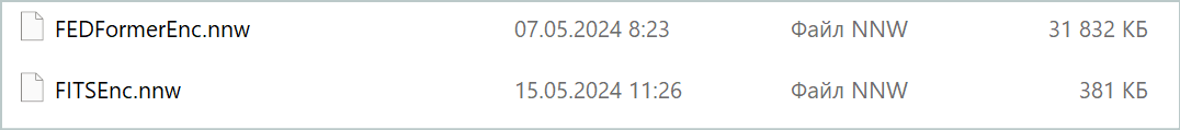
As expected, the Encoder model turned out to be quite light. The learning process is relatively fast and smooth. Despite its small size, the model demonstrates performance comparable to the FEDformer model discussed in the previous article. It is worth noting here that the size of the model is almost 84 times smaller.
But the Actor's policy training phase was disappointing. The model is capable of demonstrating profitability only in certain historical sections. In the balance graph below, beyond the test section, we see quite rapid growth in the first ten days of the month. But the second decade is losing with rare profitable trades. The third decade approaches parity between profitable and losing trades.

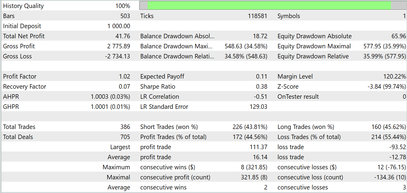
Overall, we received a small income for the month. Here it can be noted that the size of the largest and average profitable trades exceeds the corresponding loss metric. However, the number of profitable trades is less than half, which negates the superiority of the average profitable trade.
It can be noted here that the testing results partly confirm the conclusions made by the authors of the FEDformer method: as there is no clear periodicity in the input data, DFT is unable to determine the moment when the trend changes.
Conclusion
In this article, we have discussed a new FITS method for time series analysis and forecasting. The key feature of this method is the analysis and forecasting of time series in the area of frequency characteristics. Since the method uses the direct and inverse fast Fourier transform algorithm, we can operate with familiar discrete time series at the input and output of the model. This feature allows the proposed lightweight architecture to be implemented in many areas where time series analysis and forecasting is used.
In the practical part of this article, we implemented our vision of the proposed approaches using MQL5. We trained and tested models using real historical data. Unfortunately, testing did not generate the desired result. However, I would like to draw attention to the fact that the presented results are relevant only for the presented implementation of the proposed approaches. The results could be different if we used the original author's algorithm.
References
- FITS: Modeling Time Series with 10k Parameters
- A Survey of Complex-Valued Neural Networks
- Other articles from this series
Programs used in the article
| # | Name | Type | Description |
|---|---|---|---|
| 1 | Research.mq5 | Expert Advisor | Example collection EA |
| 2 | ResearchRealORL.mq5 | Expert Advisor | EA for collecting examples using the Real-ORL method |
| 3 | Study.mq5 | Expert Advisor | Model training EA |
| 4 | StudyEncoder.mq5 | Expert Advisor | Encode Training EA |
| 5 | Test.mq5 | Expert Advisor | Model testing EA |
| 6 | Trajectory.mqh | Class library | System state description structure |
| 7 | NeuroNet.mqh | Class library | A library of classes for creating a neural network |
| 8 | NeuroNet.cl | Code Base | OpenCL program code library |
Translated from Russian by MetaQuotes Ltd.
Original article: https://www.mql5.com/ru/articles/14913
Warning: All rights to these materials are reserved by MetaQuotes Ltd. Copying or reprinting of these materials in whole or in part is prohibited.
This article was written by a user of the site and reflects their personal views. MetaQuotes Ltd is not responsible for the accuracy of the information presented, nor for any consequences resulting from the use of the solutions, strategies or recommendations described.

 Connexus Helper (Part 5): HTTP Methods and Status Codes
- Free trading apps
- Over 8,000 signals for copying
- Economic news for exploring financial markets
You agree to website policy and terms of use