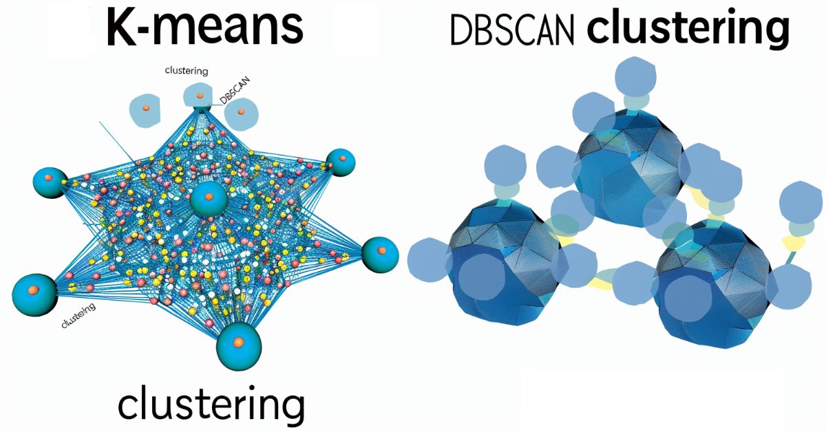
MQL5 Wizard Techniques you should know (Part 13): DBSCAN for Expert Signal Class

Introduction

These series of articles, on the MQL5 Wizard, are a segue on how often abstract ideas in Mathematics of other fields of life can be enlivened as trading systems and tested or validated before any serious commitments is made on their premise. This ability to take simple and not fully implemented or envisaged ideas and explore their potential as trading systems is one of the gems presented by the MQL5 wizard assembly for expert advisers. The expert classes of the wizard furnish a lot of the mundane features required by any expert adviser especially as it relates to opening and closing trades but also in overlooked aspects like executing decisions only on a new bar formation.

So, in keeping this library of processes as a separate aspect of an expert adviser, with the MQL5 Wizard any idea can not only be tested independently, but also compared on a somewhat equal footing to any other ideas (or methods) that could be under consideration. In these series we have looked at alternative clustering methods like the agglomerative clustering as well as the k-means clustering.

In each of these approaches, prior to generating the respective clusters, one of the required input parameters was the number of clusters to be created. This in essence assumes that the user is well versed with the data set and is not exploring or looking at unfamiliar dataset. With Density Based Spatial Clustering for Applications with Noise (DBSCAN) the number of clusters to be formed is a ‘respected’ unknown. This affords more flexibility not just in exploring unknown data sets and discovering their major classification traits, but it can also allow checking existing ‘biases’ or commonly held views on any given data set for whether the number of clusters assumed can be verified.

By taking just two parameters namely epsilon, which is the maximum spatial distance between points in a cluster; and the number of minimum points required to constitute a cluster, DBSCAN is able to not only generate clusters from sampled data, but also determine the appropriate number of these clusters. To appreciate its remarkable feats, it may be helpful to look at some clustering it can perform as opposed to alternative approaches.

According to this public article on medium, DBSCAN and k-means clustering would, by their definition give these separate clustering results. 

For k-means clustering we would have:

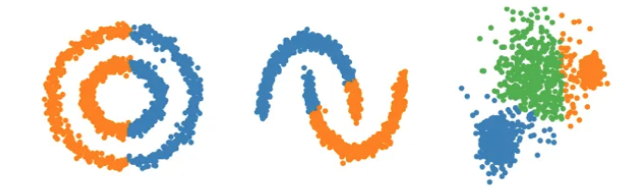
while DBSCAN would give:

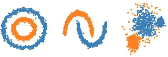
In addition to these, this paper also compared DBSCAN to another clustering approach named CLARANS that yielded the following results. For CLARANS the re-classification was:

However, DBSCAN with the same forms gave the following grouping:

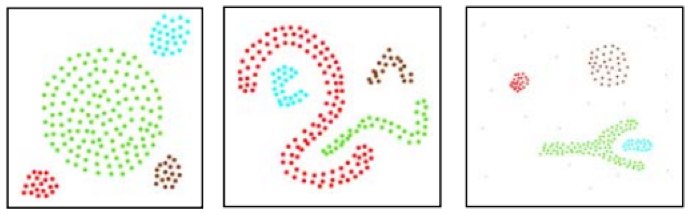
The first example may be a notional presentation however the 2nd example is definitive. The arguments behind this are that without a pre-set number of clusters required for the classification, DBSCAN uses the density or mean spacing of points to come up with appropriate groupings and therefore clusters.

As can be observed from the images above, k-means is concerned with territorial partitioning which in this case is governed by the x and y axis coordinates. So what k-means does is apportion the points within the axis constraints (in this case x & y) as a best fit. DBSCAN introduces an extra ‘dimension’ of density where it is not enough to simply abound within the coordinate axes areas but the intra-proximity of all the points also gets taken into consideration; the result of which is clusters can stretch over extended regions beyond what would be considered their average loci or best fit.

For this article therefore, we will look at how DBSCAN can help in refining buy and sell decisions of the expert signal class used in the MQL5 wizard. We have already seen how clustering can be informative in those sorts of decisions in the two prior articles on the subjects linked above, so we are going to build on that when building signal classes for DBSCAN.

To that end we will have 3 illustrations of different expert signal classes that use DBSCAN in different ways primarily from processing different data sets. Finally, as mentioned at the beginning these ideas are presented here for preliminary testing and screening and are nothing close to what should be used on live accounts. Independent diligence on the part of the reader is always expected.

Demystifying DBSCAN

In order to ‘demystify’ DBSCAN it may be a good idea to provide some illustrations, outside of trading, that we are bound to encounter on a day to day basis. So, let’s look at 3 examples.

Example-1: Imagine a situation where you are a super market owner and you have to analyze a data set on some shoppers and try to see if there are any patterns that can be gleaned and used in the future for planning purposes. This analysis again could typically take a number of forms however for our purposes we are primarily considering clustering. With k-means you would have to begin by presupposing a fixed number of types of customers let’s say you assume discretionary spenders those who only by big ticket consumer or electronic goods and only when you have a sale, and staple consumers those whom you often see in your store purchasing household groceries about once a week. With this set batching you would then proceed to itemize what they purchase and appropriately plan your inventories to be capable of handling their demand going forward. Now because you have preset your clusters (customer types) to 2 you are bound to have 2 major expenditure outlays (positioned in time as average centroids) to replenish your inventory, and this may not be as cashflow friendly as you would like since more but smaller sized expenditures could be more manageable. If on the other hand you had used DBSCAN for the segmentation of your customers then the number of types of customers you come up with would be set by their density or how close in time these customers tend to do their shopping. We had used the analogy of x and y axes in quantifying epsilon (closeness of data points) above but for the case of time with the super market customers a calendar would suffice where how ‘close’ customers are would be quantified by how far apart in time off a calendar date their shopping is. This effectively allows more flexible grouping of customers which in turn could lead to more manageable expenditure outlays when replenishing inventory among other benefits.

Example-2: Consider a situation where as an urban planner of a city you are tasked with re-assessing the maximum number of residences that should be allowed in each borough of the city from studying urban traffic patterns. Whereas in example-1 we used time as our spatial domain for the clustering, for this example we are restricted to the physical routes that traverse the city and perhaps connect the boroughs. K-means clustering would begin by using the existing number of boroughs as the clusters and then determine the weighting or population threshold of each borough based off of the average amount of morning & evening traffic in its connection routes. With the new weighting proportion each borough we would then have its residential limit reduced or increased proportionately. However, the boroughs themselves may not be cast in stone. Some may be dying, others thriving and more importantly some may be emerging thus by using DBSCAN with only the traffic routes and not assumptions on number of boroughs we can group the routes into different forms of clusters which clusters would then map our new boroughs. Our epsilon in this case would track how many cars we have on each route (in the peak morning and evening hours) on say a per kilometer basis. This could imply that more dense routes could be grouped together than less dense ones which creates problems in cases where routes lead to different geographical areas. The way to work around this or understand the data would be that those routes, even though mapping to different physical areas, represent the same ‘type of borough’ (could be due to income level etc.) and therefore for planning purposes they can be provisioned for in a similar manner.

Example-3: Finally, social networks are a gold data mine for many companies and key in understanding them better could be in the ability to classify or in our case clusterizer the users into disparate groups. Now because social media users form their own groups for leisure or work, may have shared interests or not, and may even interact sporadically; it is a herculean task for k-means to come up with an acceptable number of clusters off the bat when starting the clustering process. DBSCAN on the other hand, by focusing on density, can zero in on the number of user interactions, say through enumeration over a set time period. This number of interactions from one user to another can thus guide the epsilon parameter in forming and defining the different clusters that could be possible on a given social media platform.

Besides the points raised in these examples it is also worth noting that DBSCAN is better adept at handling noise and identifying outliers especially in situations of unsupervised learning as is the case with DBSCAN. The minimum number of points input parameter is also important when arriving at the ideal number of clusters for a sampled data set however it is not as sensitive (or important) as epsilon because its role in essence is setting the ‘noise’ threshold. With DBSCAN any data that does not fall within designated clusters is noise.

Implementing in MQL5

So, the basic structure of MQL5 wizard assembled expert advisers has already been covered in previous articles. The official primer on this can be found here. However, to recap wizard assembled expert advisers depend on the Expert Class defined in ‘<include\Expert\Expert.mqh>’ file. This expert class primarily defines how the typical expert adviser functions that relate to opening and closing of positions are handled. It in turn depends on the Expert-Base Class that is defined in the file ‘<include\Expert\ExpertBase.mqh>’ and this later file handles retrieval and buffering of current price information for the symbol the expert advisor is attached to. From the Expert Class which we can think of as the anchor, 3 other classes are derived by inheritance from it namely: the Expert Signal Class, the Expert Trailing Class and the Expert Money Class. Customized implementations of each of these classes have already been shared in previous articles however it worth reiterating that the Expert signal class handles buy and sell decisions, while the Expert Trailing Class determines when and by how much to move the trailing stop on open positions and finally the Expert Money Class sets what proportion of available margin can be used in position sizing.

The steps in assembling an expert advisor from available classes in the library are really straight forward and there are articles here besides the shared link above on how to go about this. Data preparation is handled by the Expert Base Class however for this to be bankable testing should ideally be done with price data of your intended broker and real ticks should be downloaded from their server as much as is available.

In coding the DBSCAN function this public paper shares some useful source code which we build on to define our functions. If we begin with the most basic of these, there are 4 simple functions in total, we would be looking at the distance function.

//+------------------------------------------------------------------+
//| Function for Euclidean Distance between points                   |
//+------------------------------------------------------------------+
double CSignalDBSCAN::Distance(Spoint &A, Spoint &B)
{  double _d = 0.0;
   for(int i = 0; i < int(fmin(A.key.Size(), B.key.Size())); i++)
   {  _d += pow(A.key[i] - B.key[i], 2.0);
   }
   _d = sqrt(_d);
   return(_d);
}

The cited paper and most public source code on DBSCAN use Euclidean distance as the primary metric for quantifying how far points are in any set of points. However, seeing as our points are in a vector form, MQL5 does present quite a few other alternatives to measuring this distance between points, such as cosine similarity etc. and the reader could explore these since they are sub-functions of the vector data type. We code the Euclidean function from scratch as I was unable to find it under the Loss function or Regression Metric functions.

Next up among the building blocks we need a ‘RegionQuery’ function. This returns a list of points within the threshold defined by the input parameter epsilon that can be deemed to be within the same cluster as the point in question.

//+------------------------------------------------------------------+
//| Function that returns neighbouring points for an input point &P[]|
//+------------------------------------------------------------------+
void CSignalDBSCAN::RegionQuery(Spoint &P[], int Index, CArrayInt &Neighbours)
{  Neighbours.Resize(0);
   int _size = ArraySize(P);
   for(int i = 0; i < _size; i++)
   {  if(i == Index)
      {  continue;
      }
      else if(Distance(P[i], P[Index]) <= m_epsilon)
      {  Neighbours.Resize(Neighbours.Total() + 1);
         Neighbours.Add(i);
      }
   }
   P[Index].visited = true;
}

Typically for each point within a data set under consideration, we try to come up with such a list of points, so that nothing is overlooked, and this list is useful for the next function which is the ‘ExpandCluster’ function.

//+------------------------------------------------------------------+
//| Function that extends cluster for identified cluster IDs         |
//+------------------------------------------------------------------+
bool CSignalDBSCAN::ExpandCluster(Spoint &SetOfPoints[], int Index, int ClusterID)
{  CArrayInt _seeds;
   RegionQuery(SetOfPoints, Index, _seeds);
   if(_seeds.Total() < m_min_points) // no core point
   {  SetOfPoints[Index].cluster_id = -1;
      return(false);
   }
   else
   {  SetOfPoints[Index].cluster_id = ClusterID;
      for(int ii = 0; ii < _seeds.Total(); ii++)
      {  int _current_p = _seeds[ii];
         CArrayInt _result;
         RegionQuery(SetOfPoints, _current_p, _result);
         if(_result.Total() > m_min_points)
         {  for(int i = 0; i < _result.Total(); i++)
            {  int _result_p = _result[i];
               if(SetOfPoints[_result_p].cluster_id == -1)
               {  SetOfPoints[_result_p].cluster_id = ClusterID;
               }
            }
         }
      }
   }
   return(true);
}

This function which takes a cluster ID and a point index determines whether the cluster ID needs to be assigned to any new points based on the results of the region query function already mentioned above. If the result is true then the cluster increases in size, otherwise it stays maintained. Within this function we check for already cluster identified points to avoid repetition and as stated above any un-clustered points (that keep cluster ID: -1) are deemed noise.

Putting this all together is done via the main DBSCAN function which iterates through all the points in a data set by establishing whether the current cluster ID needs to be expanded. The current cluster ID is an integer that gets incremented whenever a new cluster is established and at each increment the neighborhood of all points belonging to this cluster is queried via the region query function as already mentioned and this is called via the expand cluster function. The listing for this is below:

//+------------------------------------------------------------------+
//| Main clustering function                                         |
//+------------------------------------------------------------------+
void CSignalDBSCAN::DBSCAN(Spoint &SetOfPoints[])
{  int _cluster_id = -1;
   int _size = ArraySize(SetOfPoints);
   for(int i = 0; i < _size; i++)
   {  if(SetOfPoints[i].cluster_id == -1)
      {  if(ExpandCluster(SetOfPoints, i, _cluster_id))
         {  _cluster_id++;
            SetOfPoints[i].cluster_id = _cluster_id;
         }
      }
   }
}

Similarly, the struct that handles the data set referred to as ‘se of points’ in the above listing, is defined in the class header as follows:

   struct Spoint
   {  vector            key;
      bool              visited;
      int               cluster_id;

                     Spoint()
      {              key.Resize(0);
         visited = false;
         cluster_id = -1;
      };
                    ~Spoint() {};
   };

DBSCAN as a clustering method does face memory challenges depending on the size of the data set. Also, there is a school of thought that feels epsilon the key input parameter that measures cluster density should not be uniform for all clusters. In the implementation we are using for this article, this is the case however there are variants of DBSCAN like HDBSCAN that we may cover in future articles that do not even require epsilon as an input but only rely on the minimum number of points in a cluster which is a less critical and sensitive parameter which makes it a more versatile approach at clustering.

Signal Classes

If we build on what we’ve defined above in implementation we can present a number of different approaches at clustering security price data to generate trade signals. So, the three example approaches promised at the start of the article will be clustering:

- raw OHLC price bar data,

- changes in RSI indicator data,

- and finally changes in the Moving Average Price indicator.

In previous clustering articles we had a crude model where we posthumously labelled clustered values with eventual changes in price and used current weighted averages of these changes to make our next forecast. We will adopt a similar approach but the main difference between each method will primarily be the data set fed into our DBSCAN function. Because these data sets are varying the input parameters for each signal class may be different as well.

If we start with raw OHLC data, our data set will constitute 4 key points. So, the vector we defined as ‘key’ in the ‘Spoint’ struct that holds our data will have a size of 4. These 4 points will be the respective changes in open, high, low, and close prices. So, we populate an ‘Spoint’ struct with the current price information as follows:

//+------------------------------------------------------------------+
//|                                                                  |
//+------------------------------------------------------------------+
double CSignalDBSCAN::GetOutput()
{  double _output = 0.0;
   
...

...


   for(int i = 0; i < m_set_size; i++)
   {  for(int ii = 0; ii < m_key_size; ii++)
      {  if(ii == 0)
         {  m_model.x[i].key[ii] = (m_open.GetData(StartIndex() + i) - m_open.GetData(StartIndex() + ii + i + 1)) / m_symbol.Point();
         }
         else if(ii == 1)
         {  m_model.x[i].key[ii] = (m_high.GetData(StartIndex() + i) - m_high.GetData(StartIndex() + ii + i + 1)) / m_symbol.Point();
         }
         else if(ii == 2)
         {  m_model.x[i].key[ii] = (m_low.GetData(StartIndex() + i) - m_low.GetData(StartIndex() + ii + i + 1)) / m_symbol.Point();
         }
         else if(ii == 3)
         {  m_model.x[i].key[ii] = (m_close.GetData(StartIndex() + i) - m_close.GetData(StartIndex() + ii + i + 1)) / m_symbol.Point();
         }
      }
      if(i > 0) //assign classifier only for data points for which eventual bar range is known
      {  m_model.y[i - 1] = (m_close.GetData(StartIndex() + i - 1) - m_close.GetData(StartIndex() + i)) / m_symbol.Point();
      }
   }
   
...

   return(_output);
}

If we assemble this signal via the wizard and run tests on EURUSD for the year 2023 on the daily timeframe, our best run gives us the following report and equity curve.

From the reports you could say there is potential however in this case we have not done a walk forward test as we had attempted on a small scale in previous articles so the reader is invited to have this done before taking this any further.

Continuing with the absolute values of RSI as a data set we would implement this in a similar manner with the main difference being how we are accounting for the 3 different lag periods to which we take RSI readings. So, with this data set we are getting 4 data points per time as with the raw OHLC prices but these data points are RSI indicator values. The lags at which they are taken is set by 3 input parameters which we have labeled A, B, and C. The data set is populated as follows:

//+------------------------------------------------------------------+
//|                                                                  |
//+------------------------------------------------------------------+
double CSignalDBSCAN::GetOutput()
{  double _output = 0.0;

...

   RSI.Refresh(-1);
   for(int i = 0; i < m_set_size; i++)
   {  for(int ii = 0; ii < m_key_size; ii++)
      {  if(ii == 0)
         {  m_model.x[i].key[ii] = RSI.Main(StartIndex() + i);
         }
         else if(ii == 1)
         {  m_model.x[i].key[ii] = RSI.Main(StartIndex() + i + m_lag_a);
         }
         else if(ii == 2)
         {  m_model.x[i].key[ii] = RSI.Main(StartIndex() + i + m_lag_a + m_lag_b);
         }
         else if(ii == 3)
         {  m_model.x[i].key[ii] = RSI.Main(StartIndex() + i + m_lag_a + m_lag_b + m_lag_c);
         }
      }
      if(i > 0) //assign classifier only for data points for which eventual bar range is known
      {  m_model.y[i - 1] = (m_close.GetData(StartIndex() + i - 1) - m_close.GetData(StartIndex() + i)) / m_symbol.Point();
      }
   }
   int _o[];

...

...

   return(_output);
}

So, when we run tests for the same symbol over the same period 2023 at the daily time frame we do obtain the following results from our best run:

A promising report but once again inconclusive pending one’s own diligence. All Assembled experts for this article place trades by limit order and do not use take profit or stop loss price for closing positions. This implies positions are held until a signal reverses and then a new position is opened in reverse.

Finally, with changes in Moving Average we would fill a data set almost like we did with RSI the main difference being here we are looking for changes in the MA indicator readings whereas with RSI we were interested in the absolute values. Another major difference would be the key values, the size of the ‘key’ vector within ‘Spoint’ struct is only 3 and not 4 since we are focusing on lag changes and not absolute readings.

Performing test runs gives the following report for its best run.

Conclusion

To conclude, DBSCAN is an unsupervised way of classifying data that takes minimal input parameters unlike more conventional approaches like k-means. It requires only two parameters of which only one, epsilon, is critical and this does lead to an over dependence or sensitivity towards this input.

Despite this over-reliance on epsilon, the fact that for any classification the number of clusters is determined organically does make it quite versatile over various sets of data and better able to handle noise.

When used within a custom instance of the expert signal class a wide variety of input datasets from raw prices to indicator values can be used as the basis for classifying a security.

Besides creating a custom instance of the Expert Signal Class the reader can create similar custom implementations of the Expert Trailing class or the Expert Money Class that also use DBSCAN as we have covered in previous articles in these series.

Another avenue worth looking at which I feel is what DBSCAN and clustering in general are primed for, is data normalization. A lot of forecasting models tend to require a form of normalization of any input data before it can be used in forecasting. For instance, a Random Forest Algorithm or a Neural Network would ideally need normalized data especially if this data-feed is security prices. In the now in-vogue Large Language Models that use Transformer Architecture the equivalent step to this is embedding where essentially all text including the numeric, is re-assigned a number for purposes of feed forward processing through a neural network. Without this normalization of text and numbers it would be impossible for the network to feasibly process the vast amounts of data it does in developing AI algorithms. But also, this normalization does deal with outliers which can be a headache when trying to train a network and come up with acceptable weights and biases. There could be other pertinent uses of clustering and DBSCAN but those are my two cents. Happy hunting.