
MQL5 Wizard Techniques you should know (Part 70): Using Patterns of SAR and the RVI with a Exponential Kernel Network
Introduction
In the last article, we introduced this complimentary pair of the Parabolic SAR indicator (SAR) and the Relative Vigour Index oscillator (RVI). From our testing of 10 patterns, three failed to perform clean forward walks; namely those indexed 1, 2, and 6. Our indexing of these patterns from 0 to 9 allows us to easily compute the map value that allows their exclusive use by the Expert Advisor. For instance, if a pattern is indexed 1 then we have to set the parameter ‘PatternsUsed’ to 2 to the power 1 which comes to 2.
If the index is 2 then this is 2 to the power 2 which comes to 4, and so on. The maximum value that this parameter can be assigned, meaningfully, is 1023 since we have only 10 parameters. Any number between 0 and 1023 that is not a pure exponent of 2 would represent a combination of these patterns, and the reader could explore setting up the expert Advisor to use multiple patterns. However, based on our arguments and test results presented in past articles we choose not to explore this avenue within these series, for now.
As promised in one of the past recent articles, we are now going to attempt to resuscitate the three pattern signals 1, 2, and 6 that were not able to perform clean forward walks in the past article, with supervised learning. In applying machine learning to these MQL5 indicator signals, we resort to Python to help with coding and training a network model. This is because of the efficiencies it is able to provide, even without a GPU. When using Python, we rely on MetaTrader’s Python Module that allows us to connect to a MetaTrader Broker’s server once we provide a login username and password.
Once a connection is made via the MetaTrader 5 Python Module, we have access to a Broker’s price data. Python also has libraries for technical indicators, but they require installation and are often in slightly esoteric formats. Luckily, implementing our own from first principles is a relatively straightforward process. We therefore begin by implementing our two indicators, the SAR and RVI in Python.
Parabolic SAR (SAR) Function
The SAR is a trend following indicator used to spot possible reversal fractal points in price direction. It uses dot placement to mark a prevalent trend, with the dots being on the side of potential stop-loss points. So a bullish trend would have its dots below the lows, while a bearish trend would have them above the highs. We code the function for computing the SAR as follows:
def SAR(df: pd.DataFrame, af: float = 0.02, af_max: float = 0.2) -> pd.DataFrame:
    """
    Calculate Parabolic SAR indicator and append it as 'SAR' column to the input DataFrame.

    Args:
        df (pd.DataFrame): DataFrame with 'high', 'low', 'close' columns
        af (float): Acceleration factor, default 0.02
        af_max (float): Maximum acceleration factor, default 0.2

    Returns:
        pd.DataFrame: Input DataFrame with new 'SAR' column
    """
    if not all(col in df.columns for col in ['high', 'low', 'close']):
        raise ValueError("DataFrame must contain 'high', 'low', 'close' columns")
    if af <= 0 or af_max <= 0 or af > af_max:
        raise ValueError("Invalid acceleration factors")
    if df.empty:
        raise ValueError("DataFrame is empty")

    result_df = df.copy()
    result_df['SAR'] = 0.0

    sar = df['close'].iloc[0]
    ep = df['high'].iloc[0]
    af_current = af
    trend = 1 if len(df) > 1 and df['close'].iloc[1] > df['close'].iloc[0] else -1

    for i in range(1, len(df)):
        prev_sar = sar
        high, low = df['high'].iloc[i], df['low'].iloc[i]

        if trend > 0:
            sar = prev_sar + af_current * (ep - prev_sar)
            if low < sar:
                trend = -1
                sar = ep
                ep = low
                af_current = af
            else:
                if high > ep:
                    ep = high
                    af_current = min(af_current + af, af_max)
        else:
            sar = prev_sar + af_current * (ep - prev_sar)
            if high > sar:
                trend = 1
                sar = ep
                ep = high
                af_current = af
            else:
                if low < ep:
                    ep = low
                    af_current = min(af_current + af, af_max)

        result_df.loc[i, 'SAR'] = sar

    return result_df
Our implemented function above takes a pandas data frame with high, low, and close price columns as well as two float parameters for the acceleration factor. The output in the end appends the computed values as a column to the input data frame as a new column labelled ‘SAR’. Its overall logic is meant to track trend direction and update the SAR, basing on the extreme point and acceleration factor.
If we look at the code details, we start by creating a copy of the input data frame to avoid performing a modification on the original. This extracts the high, and low data columns as NumPy arrays for efficient computation. We then initialize the ‘sar’ array with zeroes to store ‘sar’ values. This is important because it ensures data integrity and prepares the structure for SAR computations. Use of `.copy()’ does prevent unintended side effects. NumPy arrays also tend to give better performance when compared to pandas series when doing iterative calculations.
After this, we set the starting trend as an uptrend with trend = 1. The extreme point is also assigned to the starting high, and the beginning SAR is also given the initial low price. The acceleration factor begins with the input value ‘af-start’. This is vital because it defines a beginning point for the SAR computations, by assuming an initial uptrend. The choice of the low[0] value for the starting SAR does align with the SAR’s role as a stop-loss to an uptrend, since it is below the low price by the ‘af-start’ parameter weight that adjusts its subtraction from the low in line with market volatility.
We then proceed to update the SAR formula. The updates provided are for the current period by moving it closer to the extreme point as scaled by the acceleration factor. This is important since it is core to the SAR formula. A parabolic offsetting of price as a trend unfolds. It is important to ensure when implementing this that ‘af’ is small so as not to have a very aggressive stepping once a trend picks up. It is also crucial to monitor for numerical stability in volatile markets.
With this done, we proceed to set the trend reverse logic. When experiencing an uptrend and the SAR exceeds the current low, a reversal to the downtrend is done. The SAR gets a reset to the previous extreme point, and the new extreme point is set to the current low. The acceleration factor also gets readjusted to its default value.
This is important because trend reversal detection is a key feature for the SAR in signalling entry/exit points. This condition ensures the SAR stays below the price in an uptrend. Testing for reversal sensitivity can be done by adjusting the ‘af-increment’ parameter.
If we are in a continuing bullish situation, then we need to still update our SAR buffer values and more importantly increment the ‘af-increment’. The SAR remains capped at the minimum of the current value or the last two lows in order to prevent it from encroaching on the price range. Also, once the high exceeds the extreme point, the extreme point gets updated while the acceleration factor also receives an increment provided it does not exceed its cap, set by ‘af-max’. This maintenance step is important because it ensures SAR remains a valid stop-loss level and only accelerates in tandem with the trend. The use of two previous lows does bring some robustness, however it may require some adjustment when facing smaller timeframes.
The downtrend/bearish logic of the SAR also gets set next. In many ways, this mirrors the uptrend/ bullish logic we’ve just mentioned. To recap, if SAR falls below the current high, it reverses to an uptrend. If no reversal happens, the SAR remains capped at the maximum of the current SAR and the prior highs. The extreme point as well as the acceleration factor do receive an update. This step completes SAR’s ability to track both uptrends and downtrends symmetrically. It is always important to ensure symmetry in uptrend and downtrend logic in order to avoid any bias. Validation can be performed on historical data to confirm the reversal accuracies.
With the SAR logic addressed, we proceed to the output assignment. Essentially, this provides the calculated SAR values to a new ‘SAR’ column in the data frame and then returns it. This is key because it integrates the indicator into the data frame to allow further analysis or visualization. When in use, it may be a good idea to verify that the SAR column aligns with price data. This can be done by using plotting libraries such as Matplotlib to visualize the SAR dots.
To sum up the SAR, it is best suited for trending markets where it can help with signalling stop-loss levels, and identifying reversal points. It would not work well in sideways or choppy markets. Parameter tuning, though not as critical for the SAR, can be important for some assets as the acceleration factor start and increment can need adjustment from their comfort values of 0.02, and 0.2. Validation by back test against broker historical data can be resourceful. Main SAR limitations are its tendency to lag in fast-moving markets, which can generate many false signals.
Relative Vigour Index (RVI) Function
The main objective of the RVI is to track the strength of a trend, something which we take to be synonymous with momentum. This is done by comparing the closing price’s position relative to the trading range and smoothing this with moving averages. It is an oscillator that can serve to confirm trend by checking momentum or by spotting divergences. We implement it in Python as follows:
def RVI(df: pd.DataFrame, period: int, signal_period: int) -> pd.DataFrame:
    """
    Calculate Relative Vigor Index (RVI) with signal line and append as 'RVI' and 'RVI_Signal' columns.

    Args:
        df (pd.DataFrame): DataFrame with 'open', 'high', 'low', 'close' columns
        period (int): Lookback period for RVI calculation
        signal_period (int): Lookback period for signal line calculation

    Returns:
        pd.DataFrame: Input DataFrame with new 'RVI' and 'RVI_Signal' columns
    """
    # Input validation
    if not all(col in df.columns for col in ['open', 'high', 'low', 'close']):
        raise ValueError("DataFrame must contain 'open', 'high', 'low', 'close' columns")
    if period < 1 or signal_period < 1:
        raise ValueError("Period and signal period must be positive")

    # Create a copy to avoid modifying the input DataFrame
    result_df = df.copy()

    # Calculate price change and range
    close_open = df['close'] - df['open']
    high_low = df['high'] - df['low']

    # Calculate SMA for numerator and denominator
    num = close_open.rolling(window=period).mean()
    denom = high_low.rolling(window=period).mean()

    # Calculate RVI
    result_df['RVI'] = num / denom * 100

    # Calculate signal line (SMA of RVI)
    result_df['RVI_Signal'] = result_df['RVI'].rolling(window=signal_period).mean()

    return result_df
From our code above, in general, we are taking a pandas data frame with the data columns ‘high’, ‘low’ and ‘close’. In addition, the inputs include a ‘period’ for the signal buffer’s SMA moving average. The output appends the RVI, that has been smoothed together with an RVI signal, to the columns of the data frame. Basically, the logic calculates RVI as close - open/high - low. This then gets smoothed with a 4-period SMA, and we generate a signal line with a user defined SMA period.
If we now consider this line by line, the first thing we are doing in our function is make a copy of the input data frame. This serves as a way of preserving the original data. It is important as we are able to avert unintended modifications to the input data frame. The use of the copy function easily helps us achieve this and avoid unintended ‘side effects’.
Next we calculate the RVI. This computation of the raw RVI sets it as a ratio of the price change to the trading range. It is important since it captures the vigour of price movement relative to the day’s range, and this forms the basis of the RVI. It is important to ensure that the ‘high’ and ‘low’ are not equal in order to avoid zero divides. This problem, though, is addressed in the next step. For now, the formula assumes intraday momentum.
To handle errors from zero division, we replace infinite values, from a possible zero division above when the high is equal to the low, with NaN. Each Nan then gets replaced by zero. This is important to ensure numerical stability and also prevent errors in subsequent calculations. For guidance, this is a simplistic fix as the reader can consider alternative handling approaches in the event that the zero values overly distort the RVI output buffer.
With this, we proceed to smooth the RVI and also define the signal line. The smoothing applies a 4-period SMA on the raw RVI to reduce susceptibility to noise and even the odd zero values that may be encountered as mentioned above. This helps create the indicator RVI line. Once this is set, we also apply a user defined period SMA to extra-smooth this already smoothed RVI in order to generate the signal line. This whole step is vital, as smoothing makes the RVI more interpretable. The signal line as well helps us more definitively spot the cross-overs of implementation of this often uses the fixed 4-period SMA in smoothing the raw RVI, however there is always room for adjusting the signal period SMA if fine-tuning is a requirement. Periods in the range 6-14 can be considered.
With this done, the output then gets assigned. The smoothed RVI and the signal line RVI each get allotted data columns on the output data frame. This, on paper, allows for both the RVI and its signal buffer to partake in further analysis or visualizations. Plotting of both buffers can help highlight cross-overs, for instance.
To sum up, the RVI is applied in confirming trend strength by serving as a momentum proxy. It can also pinpoint divergences early on, such as when price is making new highs while the RVI is not. Also, crossovers with its signal line help second bullish or bearish outlooks. Parameter tuning for the RVI primarily evolves around adjusting the ‘period’ for the SMA used in smoothing RVI for the signal line. Shorter periods in the 6 region can be used for faster/ frequent signals, while periods that are about 14 serve for smoother signals. Validation by testing RVI crosses and divergences on historical data is important in establishing signal reliability. Main RVI limitations are its ability to lag due to the double smoothing that it uses. It can also struggle to generate meaningful signals in low-volatility markets.
SAR RVI Complementarity
This indicator pairing, as with most that we have considered for this series, is selected because each indicator compliments the other. The SAR is a trend following indicator plotted on a price chart. However, the RVI is an oscillator plotted in a separate window from the price chart and used primarily to measure momentum. SAR is better positioned to set stop-losses, while the RVI is better off confirming trends or identifying divergences.
Both are implemented in Python by relying on pandas for data handling. NumPy role is in speeding up computations. SAR’s logic, which is iterative, tends to be more complex because of trend reversals. RVI’s vectorized operations on the other hand are more simple, however they are susceptible to zero-division scenarios. The performance of this indicator duo is therefore boosted by NumPy arrays use for SAR given the use of iterative calculations and by pandas' data frames when handling the vectorized RVI.
Further measures that the reader can choose to implement for this pairing can involve back testing in Python with libraries like zipline; visualization, especially for manual traders, of the SAR dot plots as well as the RVI with its signal line; error handling by supplementing the above code with input validation such as checking that the required data columns are present in the pandas data frame or that indicator period is valid; and finally extensions can be added for each indicator. For instance, the RVI supplement with divergence detection, or it could employ alternative smoothing methods.
Selected Signal Patterns
Feature-1
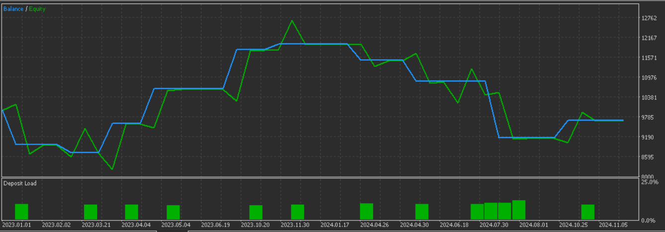
Most patterns in the last article were able to provide some form of forward walk, however the patterns indexed 1, 2, and 6 did not. In the past, we have been dwelling on patterns that forward walked by exploring if machine learning can further sharpen their edge. However for this article, and probably many to follow like it, we will be using machine learning to attempt to reverse the fortunes of patterns that are unable to forward walk following the preliminary testing.
In Python, much like in MQL5, each of these patterns needs to be assigned a function that outputs its signal of either true or false. True if the pattern signal is present, and false if not. These true or false outputs are cast as binary signals of 0s and 1s, since they bring together trading strategies of two indicators and price data. Each function creates a feature array with two columns. The first column, column-0, registers bullish signals. The second column, column-1 then logs the bearish. For each column, a 0 is logged for a no signal and a 1 for a present signal.
As already introduced in the last article, feature-1 detects trends when price stays above/ below the SAR and at the same time RVI is rising/ falling. It dwells on a sustained SAR-price symbiosis as well as RVI momentum. We implement this function in Python as follows:
def feature_1(sar_df, rvi_df, price_df):
    """

    """
    feature = np.zeros((len(sar_df), 2))

    feature[:, 0] = ((price_df['low'].shift(1) > sar_df['SAR'].shift(1)) &
                     (price_df['low'] > sar_df['SAR']) &
                     (rvi_df['RVI'] > rvi_df['RVI'].shift(1))).astype(int)

    feature[:, 1] = ((price_df['high'].shift(1) < sar_df['SAR'].shift(1)) &
                     (price_df['high'] < sar_df['SAR']) &
                     (rvi_df['RVI'] < rvi_df['RVI'].shift(1))).astype(int)


    feature[0, :] = 0
    feature[1, :] = 0

    return feature
The first thing we do in our code above is to initialize a zero-filled array to have the shape [length of the input data frames, 2]. The assigned 2 ‘columns’ at the end are meant to capture bullish and bearish signals respectively. This step is important as it ensures a clean slate for keeping our binary signals and avoids having un-initialized values. The use of np.zeros is for efficiency and works to prevent unexpected results in the numerical operations, since NaN values can automatically be used to fill a blank array as well.
With initialization done, we set the value for the bullish signal. For column 0, we assign a 1 if the previous low is over the current SAR in sustained bullish trend; and the current low is also over the SAR; with the current RVI above the prior reading indicating rising momentum. Using ALL these signals is important in grabbing a strong bullish trend, as confirmed by both the SAR for trend and RVI for momentum. It is important to ensure, when doing this, that `shift(1)’ aligns data correctly. Missing data can lead to major errors. The use of ‘astype(int)’ helps convert boolean values to binary, 0s and 1s.
Once the bullish column is set, we move on to assign the bearish. The bearish requirements mirror the bullish, so it is unlikely to get a feature vector with 1s in the bullish and bearish columns. Also, our feature vector size is restricted to 2 in order to only capture ‘complete’ bullishness or ‘complete’ bearishness. We have talked about and actually implemented vectors that are much longer and handle the individual indicator signals at each index. Tests with these conditions did not forward walk well, without very limited test window, and based on this we are sticking to the 2 size option of bullishness and bearishness.
So, for the second column, we set the bearish signal when the prior high is below the prior SAR and the current high is also below the current SAR. This plays out when the current RVI is lower than the prior RVI, a sign of falling momentum. All these patterns unify to define a strong bearish trend thanks to the complementarity of the SAR and RVI. Similar to the bullish logic above, we need to check for data alignment and also handle NaN values from ‘shift’.
With the bullish and bearish signals defined, we proceed to make adjustments to our output array by taking account for the shift comparisons. This we do by assigning 0s to the first two rows in order to avoid invalid signals. It is also important in preventing spurious signals from incomplete data at the beginning. As a rule, it is always good to nullify initial rows when using lagged data to keep robustness. The test results, that spanned the training and forward walk, give us the following report:
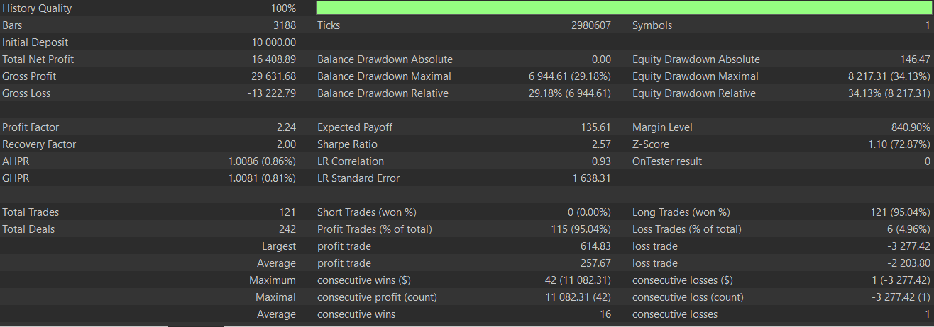
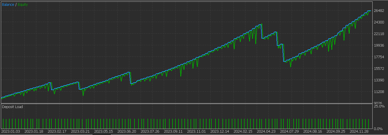
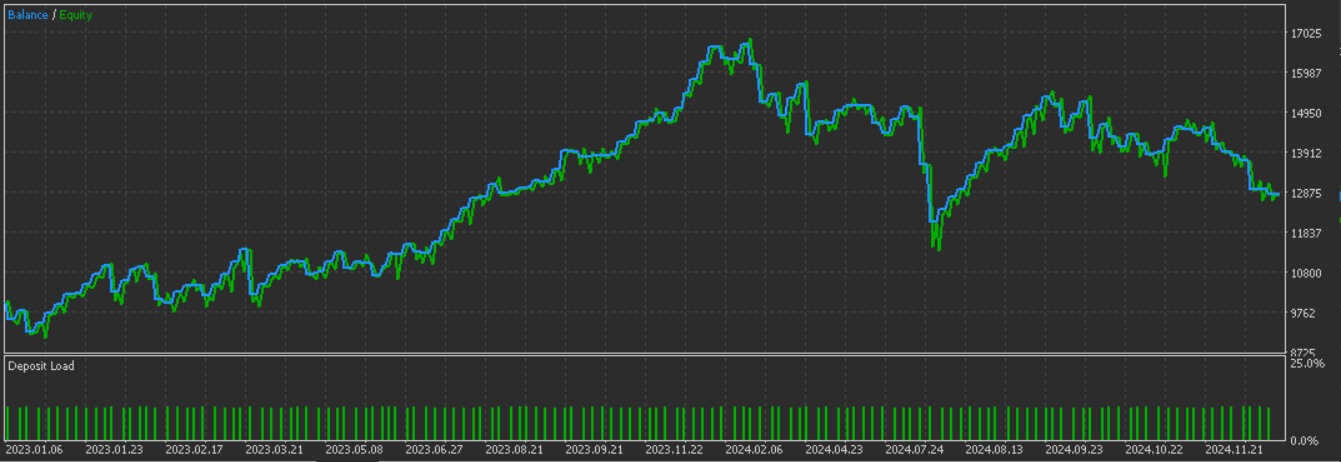
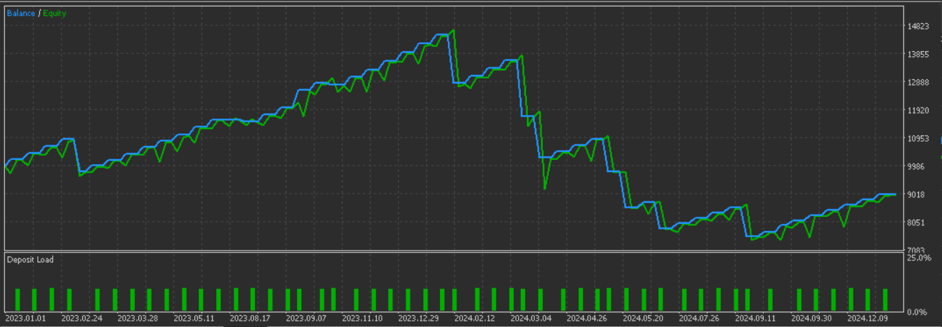
It appears we are getting better results with the introduction of supervised learning. Below is the graph we got for pattern-1 without supervised learning:
Feature-2
The third pattern we tested also failed to forward walk. This feature pattern, as was discussed in the last article, detects potential reversals where price crosses SAR and the RVI shows some momentum. It also incorporates price movement direction, by using the close price, for additional direction. We implement this in python as follows:
def feature_2(sar_df, rvi_df, price_df):
    """

    """
    feature = np.zeros((len(sar_df), 2))

    feature[:, 0] = ((price_df['high'].shift(1) <= sar_df['SAR'].shift(1)) &
                     (price_df['low'] >= sar_df['SAR']) &
                     (rvi_df['RVI'] > rvi_df['RVI'].shift(1)) &
                     (price_df['close'].shift(1) > price_df['close'])).astype(int)

    feature[:, 1] = ((price_df['low'].shift(1) >= sar_df['SAR'].shift(1)) &
                     (price_df['high'] <= sar_df['SAR']) &
                     (rvi_df['RVI'].shift(1) > rvi_df['RVI']) &
                     (price_df['close'] > price_df['close'].shift(1))).astype(int)


    feature[0, :] = 0
    feature[1, :] = 0

    return feature
We also start here by initializing a zero filled array that is shaped to receive both bullish and bearish signals. Reasons for this, as mentioned above, ensure we have no NaNs at the onset, and we can get a predictable output from the function. Consistent initialization is vital for downstream processing.
We then proceed to define the conditions for a bullish signal. All these conditions have to be met for us to register a 1 otherwise a zero is assigned. That's why working with zero-filled arrays is a safe way of avoiding false entries. So, if the previous high is at or below the prior SAR; and the current low is at or above the current SAR meaning we’ve had a flip; with the RVI is rising; and finally the close price is decreasing to affirm the divergence context. This helps capture bullish reversals where price breaks above SAR with RVI momentum. Several requirements are in play for this pattern, and all need to be confirmed before we assign the true or 1 value.
For the bearish conditions, we set these on the second index of the feature NumPy array. For a bearish value, the previous low is at or below the prior SAR; the current high is at or below the current SAR; the RVI is falling; and the close price is rising as a confirmation of the divergence setup. Signal pattern-2 spots bearish divergence, and it's important to ensure data consistency across data frames. We then nullify the initial rows of our features array by assigning zeroes in order to account for the use of shift comparisons. This prevents invalid signals from missing lagged data. It is a standard practice for time-series features’ that have lags.
This feature-2, in theory, could be used in conjunction with signal pattern-1 above because there is a bit of a complementary relationship. Feature-1 is purely a trend following system, while feature-2 targets reversals at divergence points, which can therefore bring swing trading to the fold for a more robust system. However, as argued and shown in past articles, pairing different patterns is bound to lead to the premature cross-cancelling of signals and therefore the testing for such a system needs to be with an extensive amount of history and the forward walks should also be definitive. Training and testing this pattern gives us the report below that spans both train and test periods. Again, it appears we are getting more favourable results with the use of machine learning:

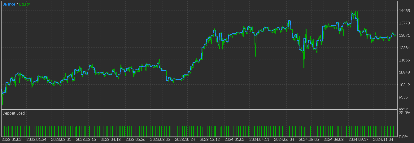
Below is the graph we got for pattern-2 without the supervised learning:
Feature-6
Our final test feature from the original 10 of the last article is based on the signal pattern-6. This uses the RVI crossover with its signal line instead of just the RVI momentum for confirmation. It focuses on strong trend signals that have SAR and RVI crossover events. We implement this in Python as follows:
def feature_6(sar_df, rvi_df, price_df):
    """

    """
    feature = np.zeros((len(sar_df), 2))

    feature[:, 0] = ((price_df['low'].shift(1) > sar_df['SAR'].shift(1)) &
                     (price_df['low'] > sar_df['SAR']) &
                     (rvi_df['RVI'] > rvi_df['RVI_Signal']) &
                     (rvi_df['RVI'].shift(1) < rvi_df['RVI_Signal'].shift(1))).astype(int)

    feature[:, 1] = ((price_df['high'].shift(1) < sar_df['SAR'].shift(1)) &
                     (price_df['high'] < sar_df['SAR']) &
                     (rvi_df['RVI'] < rvi_df['RVI_Signal']) &
                     (rvi_df['RVI'].shift(1) > rvi_df['RVI_Signal'].shift(1))).astype(int)

    feature[0, :] = 0
    feature[1, :] = 0

    return feature
We begin as always with sizing a zero filled NumPy array to hold our intended outputs. This initialization is important and consistent with the other functions in ensuring a clean NaN free output. It also helps maintain the predictable array structure for downstream use.
With this done, we define the conditions for the bullish signal which are logged at the first index, zero. We register a 1 if the previous low is above the SAR; and the current low is above the current SAR; and the current RVI is also above its signal line; and finally the prior RVI was below its signal.
With the bullish pattern defined, we also establish the bearish, which is when the prior high is below the prior SAR; and this is maintained by the current high also being below the current SAR; and the current RVI is below its signal line; with the previous RVI having been above the zero bound. Training and testing this pattern as with the other two gives us the following test report. Once again it appears we have a favourable forward walk.

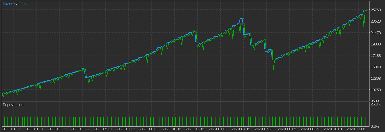
Below is the graph we got for pattern-6 without supervised learning:
The Network
In testing, our select 3 patterns above, we have engaged a neural network that is a 1D Convolutional Neural Network. It has three convolutional layers, with each increasing their filter counts and kernel sizes exponentially. This is followed by max-pooling, which is a flattening operation. Finally, we employ the fully connected layers to work our way to the final output. This we code as follows in Python:
class ExpConv1DNetwork(nn.Module):
    def __init__(self, input_length, input_channels=1, base_filters=16, base_kernel_size=3, exp_base=2):
        super(ExpConv1DNetwork, self).__init__()
        self.conv_layers = nn.ModuleList()
        self.pool_layers = nn.ModuleList()

        for i in range(3):
            filters = int(base_filters * (exp_base ** i))
            kernel_size = int(base_kernel_size * (exp_base ** i)) | 1
            self.conv_layers.append(
                nn.Conv1d(
                    in_channels=input_channels if i == 0 else int(base_filters * (exp_base ** (i-1))),
                    out_channels=filters,
                    kernel_size=kernel_size,
                    padding='same'
                )
            )
            # Use smaller kernel size for pooling to prevent size reduction to 0
            self.pool_layers.append(nn.MaxPool1d(kernel_size=2, ceil_mode=True))

        self.flatten_size = self._get_flatten_size(input_length, input_channels, base_filters, exp_base)
        self.flatten = nn.Flatten()
        self.dense1 = nn.Linear(self.flatten_size, 128)
        self.relu = nn.ReLU()
        self.dropout = nn.Dropout(0.5)
        self.dense2 = nn.Linear(128, 1)

    def _get_flatten_size(self, input_length, input_channels, base_filters, exp_base):
        current_length = input_length
        current_channels = input_channels

        for i in range(3):
            current_channels = int(base_filters * (exp_base ** i))
            # Update length after pooling
            current_length = (current_length + 1) // 2  # Ceiling division for ceil_mode=True

        return current_channels * current_length

    def forward(self, x):
        for conv, pool in zip(self.conv_layers, self.pool_layers):
            x = self.relu(conv(x))
            x = pool(x)
        x = self.flatten(x)
        x = self.relu(self.dense1(x))
        x = self.dropout(x)
        x = self.dense2(x)
        return x
This network expects a 1D input that is shaped batch-size, input-channels, input-length. It is further customizable via parameters like base-filters, base-kernel-size, and exp-base. Our output is a single scalar output trained to be in the 0 to 1 range, with 0 forecasting bearishness and 1 projecting bullishness. A blow-by-blow perusal of this class code lines would certainly have been in order, as this class is key in setting the performance of our revamped signal patterns. This however is shelved for now, given our article length, but will be something we will be mindful of in similar articles going forward.
Conclusion
We have explored potential benefits of adding supervised learning to signal patterns that were unable to perform forward walks when dealing with a limited data window of the pair GBP CHF of only 2 years. From our testing, again in very constrained conditions, it appears there is a positive difference from what we got in the last article. This is encouraging. However, as always, independent and more exhaustive diligence is always required on the part of the reader before any ideas presented here can be taken on.
| name | description |
|---|---|
| WZ-70.mq5 | File whose header indicates files used in the Wizard Assembly |
| SignalWZ_70.mqh | Custom Signal Class file, used by the MQL5 Wizard |
| 70_1.onnx | Exported network model for pattern-1 |
| 70_2.onnx | Exported network model for pattern-2 |
| 70_6.onnx | Exported network model for pattern-6 |
Warning: All rights to these materials are reserved by MetaQuotes Ltd. Copying or reprinting of these materials in whole or in part is prohibited.
This article was written by a user of the site and reflects their personal views. MetaQuotes Ltd is not responsible for the accuracy of the information presented, nor for any consequences resulting from the use of the solutions, strategies or recommendations described.
 From Novice to Expert: Animated News Headline Using MQL5 (I)
 From Basic to Intermediate: Array (IV)
 Mastering Log Records (Part 8): Error Records That Translate Themselves
 Developing a Replay System (Part 72): An Unusual Communication (I)
- Free trading apps
- Over 8,000 signals for copying
- Economic news for exploring financial markets
You agree to website policy and terms of use