MQL5 Wizard Techniques you should know (Part 09): Pairing K-Means Clustering with Fractal Waves

Introduction

This article continues the look at possible simple ideas that can be implemented and tested thanks to the MQL5 wizard, by delving into k-means clustering. This like AHC which we looked at in this prior article, is an unsupervised approach to classifying data.

So just before we jump in it may help to recap what we covered under AHC and see how it contrasts with k-means clustering. The Agglomerative Hierarchical Clustering algorithm initializes by treating each data point in the data set to be classified, as a cluster. The algorithm then iteratively merges them into clusters depending on proximity, iteratively. Typically, the number of clusters would not be pre-determined but the analyst could determine this by reviewing the constructed dendrogram which is the final output when all data points are merged into a single cluster. Alternatively, though, as we saw in that article if the analyst has a set number of clusters in mind then the output dendrogram will terminate at the level/ height where the number of clusters matches the analyst’s initial figure. In fact, different cluster numbers can be obtained depending on where the dendrogram is cut.

K-means clustering on the other hand starts by randomly choosing cluster centers (centroids) based on a pre-set figure by the analyst. The variance of each data point from its closest center is then determined and adjustments are made iteratively to the center/ centroid values until the variance is at its smallest for each cluster.

By default, k-means is very slow and inefficient in fact, that’s why it is often referred to as naïve k-means, with the ‘naïve’ implying there are quicker implementations. Part of this drudgery stems from the random assignment of the initial centroids to the data set during the start of the optimization. In addition, after the random centroids have been selected, Lloyd’s algorithm is often employed to arrive at the correct centroid and therefore category values. There are supplements & alternatives to Lloyd’s algorithm and these include: Jenks’ Natural Breaks which focuses on cluster mean rather than distance to chosen centroids; k-medians which as the name suggests uses cluster median and not centroid or mean, as the proxy in guiding towards the ideal classification; k-medoids that uses actual data points within each cluster as a potential centroid thereby being more robust against noise and outliers, as per Wikipedia; and finally fuzzy mode clustering where the cluster boundaries are not clear cut and data points can and do tend to belong to more than one cluster. This last format is interesting because rather than ‘classify’ each data point, a regressive weight is assigned that quantifies by how much a given data point belongs to each of the applicable clusters.

Our objective for this article will be to showcase one more type of k-means implementation that is touted to be more efficient and that is k-means++. This algorithm relies on Lloyd’s methods like the default naïve k-means but it differs in the initial approach towards the selection of random centroids. This approach is not as ‘random’ as the naïve k-means and because of this, it tends to converge much faster and more efficiently than the latter.

Algorithm Comparison

K-means vs K-Medians

K-means minimizes the squared Euclidean distances between cluster points and their centroid while k-medians minimizes the sum of the absolute distances of points from their median within a given cluster (L1-Norm). This distinction it is argued, makes k-medians less susceptible to outliers and it makes the cluster better representative of all the data points since the cluster center is the median of all points rather than their mean. The computation approach is also different as k-medians relies on algorithms based on L1-Norm, while k-means uses k-means++ and Lloyd’s algorithm. Use cases therefore see k-means as more capable of handling spherical or evenly spread out data sets while k-medians can be more adept at irregular and oddly shaped data sets. Finally, k-medians also tend to be preferred when it comes to interpretation since medians tend to be a better representative of a cluster than their means.

K-means vs Jenks-Natural-Breaks

The Jenks-Natural-Breaks algorithm like k-means seeks to minimize the data point to centroid distance as much as possible, where the nuanced difference lies in the fact that this algorithm also seeks to draw these classes as far apart as possible so they can be distinct. This is achieved by identifying ‘natural-groupings’ of data. These ‘natural groupings are identified within clusters at points where the variance increases significantly, and these points are referred to as breaks which is where the algorithm gets its name. The breaks are emphasized by minimizing the variance within each cluster. It is better suited for classification style data sets rather than regressive or continuous types. With all this, like the k-Median algorithm, it gains advantages in sensitivity to outliers as well as overall interpretation when compared to the typical k-means.

K-means vs K-Medoids

As mentioned K-medoids relies on the actual data rather than notional centroid points initially. In this respect, it is much like Agglomerative Hierarchical Classification but no dendrograms get drawn up here. The selected data points that are used as centroids are those with the least distance to all other data points within the cluster. This selection can also employ a variety of distance measuring techniques that include the Manhattan distance or Cosine similarity. Since centroids are actual data points it can be argued that like Junks, and K-Medians they are more representative of their underlying data than k-means however they are more computationally inefficient especially when handling large data sets.

K-means vs Fuzzy-Clustering

Fuzzy clustering as mentioned provides a regressive weight to each data point, which would be in vector format depending on the number of clusters in play. This weight would be in the 0.0 – 1.0 range for each cluster by using a fuzzy prototype (membership function) unlike k-means which uses a definitive centroid. This tends to provide more information and is therefore better representative of the data. It does out-score typical k-means on all the points mentioned above with the main drawback being on computation that is bound to be intense as one would expect.

K-means++

To make naïve k-means clustering more efficient, typically and for this article, k-means++ initialization is used where the initial centroids are less random but are more proportionately spread out across the data. This from testing has led to much faster solutions and convergence to the target centroids. Better cluster quality overall is achieved and less sensitivity to not just outlier data points but also the initial choice of centroid points.

Data

As we implemented with the article on Agglomerative Hierarchical Clustering, we’ll use AlgLib’s K-means ready classes to develop a simple and similar algorithm to what we had for that article and see if we can get a cross validated result. The security to be tested is GBPUSD, and we run tests from 2022.01.01 up to 2023.02.01 and then perform walk forwards from that date up to 2023.10.01. We will use the daily time frame and perform final runs on real ticks over the test period.

Struct

The data struct used to organize the clusters is identical to what we had in the AHC article and in fact the procedure and signal ideas used are pretty much the same. The main difference is that when we used Agglomerative clustering we had to run a function to retrieve the clusters at the level that matches our target cluster number and so we called the function ‘ClusterizerGetKClusters’ which we do not do here. Besides this we had to be extra careful and ensure the struct actually receives price information, and to this end we check a lot for invalid numbers as can be seen in this brief snippet below:

      double _dbl_min=-1000.0,_dbl_max=1000.0;
      
      for(int i=0;i<m_training_points;i++)
      {
         for(int ii=0;ii<m_point_features;ii++)
         {
            double _value=m_close.GetData(StartIndex()+i)-m_close.GetData(StartIndex()+ii+i+1);
            if(_dbl_min>=_value||!MathIsValidNumber(_value)||_value>=_dbl_max){ _value=0.0; }
            m_data.x.Set(i,ii,_value);
            matrix _m=m_data.x.ToMatrix();if(_m.HasNan()){ _m.ReplaceNan(0.0); }m_data.x=CMatrixDouble(_m);
         }
         
         if(i>0)//assign classifier only for data points for which eventual bar range is known
         {
            double _value=m_close.GetData(StartIndex()+i-1)-m_close.GetData(StartIndex()+i);
            if(_dbl_min>=_value||!MathIsValidNumber(_value)||_value>=_dbl_max){ _value=0.0; }
            m_data.y.Set(i-1,_value);
            vector _v=m_data.y.ToVector();if(_v.HasNan()){ _v.ReplaceNan(0.0); }m_data.y=CRowDouble(_v);
         }
      }

ALGLIB

The AlgLib library has already been referred to a lot in these series so we’ll jump right to the code on forming our clusters. Two functions in the library will be our focus, the ‘SelectInitialCenters’ that is crucial in expediting the whole process because as mentioned a too random initial selection of clusters tends to lengthen how long converge to the right clusters. Once this function is run we will then be using the Lloyd algorithm to fine tune the initial cluster selection and for that we turn to the function ‘KMeansGenerateInternal’.

The selection of initial clusters with available function can be done in one of 3 ways, either it is done, randomly, or with k-means++, or with fast-greedy initialization. Let’s briefly go over each. With random cluster selection as in the other 2 cases, the output clusters are stored in an output matrix named ‘ct’ whereby each row represents a cluster such that the number of rows of ‘ct’ matches the intended cluster number while the columns would be equal to the features or the vector cardinal of each data point in the data set. So, the random option simply assigns, once, to each row of ‘ct’ a data point chosen at random from the input data set. This is indicated below:

//--- Random initialization
   if(initalgo==1)
     {
      for(i=0; i<k; i++)
        {
         j=CHighQualityRand::HQRndUniformI(rs,npoints);
         ct.Row(i,xy[j]+0);
        }
      return;
     }

With K-means++ we also start by choosing a random center but only for the first cluster unlike before where we did this for all clusters. We then measure the distance between each data set point and the randomly chosen cluster center, logging the squared sum of these distances for each row (or potential cluster) and in the event that this sum is zero, we simply choose a random centroid for that cluster. For all non-zero sums stored in the variable ‘s’ we choose the point furthest from our randomly chosen initial cluster. The code is fairly complex but this is brief snippet with comments could shed more light:

//--- k-means++ initialization
   if(initalgo==2)
     {
      //--- Prepare distances array.
      //--- Select initial center at random.
      initbuf.m_ra0=vector<double>::Full(npoints,CMath::m_maxrealnumber);
      ptidx=CHighQualityRand::HQRndUniformI(rs,npoints);
      ct.Row(0,xy[ptidx]+0);
      //--- For each newly added center repeat:
      //--- * reevaluate distances from points to best centers
      //--- * sample points with probability dependent on distance
      //--- * add new center
      for(cidx=0; cidx<k-1; cidx++)
        {
         //--- Reevaluate distances
         s=0.0;
         for(i=0; i<npoints; i++)
           {
            v=0.0;
            for(j=0; j<=nvars-1; j++)
              {
               vv=xy.Get(i,j)-ct.Get(cidx,j);
               v+=vv*vv;
              }
            if(v<initbuf.m_ra0[i])
               initbuf.m_ra0.Set(i,v);
            s+=initbuf.m_ra0[i];
           }
         //
         //--- If all distances are zero, it means that we can not find enough
         //--- distinct points. In this case we just select non-distinct center
         //--- at random and continue iterations. This issue will be handled
         //--- later in the FixCenters() function.
         //
         if(s==0.0)
           {
            ptidx=CHighQualityRand::HQRndUniformI(rs,npoints);
            ct.Row(cidx+1,xy[ptidx]+0);
            continue;
           }
         //--- Select point as center using its distance.
         //--- We also handle situation when because of rounding errors
         //--- no point was selected - in this case, last non-zero one
         //--- will be used.
         v=CHighQualityRand::HQRndUniformR(rs);
         vv=0.0;
         lastnz=-1;
         ptidx=-1;
         for(i=0; i<npoints; i++)
           {
            if(initbuf.m_ra0[i]==0.0)
               continue;
            lastnz=i;
            vv+=initbuf.m_ra0[i];
            if(v<=vv/s)
              {
               ptidx=i;
               break;
              }
           }
         if(!CAp::Assert(lastnz>=0,__FUNCTION__": integrity error"))
            return;
         if(ptidx<0)
            ptidx=lastnz;
         ct.Row(cidx+1,xy[ptidx]+0);
        }
      return;
     }

As always AlgLib does share some public documentation so this can be a reference for any further clarification.

Finally, for the fast-greedy initialization algorithm that was inspired by a variant of k-means called k-means++, a number of rounds are performed where for each round: calculations for the distance closest to the currently selected centroid are made; then independent sampling of roughly half the expected cluster size is done where probability of selecting a point is proportional to its distance from current centroid with this repeated until the number of sampled points is twice what would fill a cluster; and then with the extra-large sample selected ‘greedy-selection’ is performed from this sample until the smaller sample size is attained with priority given to the points furthest from the centroids. A very compute intense and convoluted process whose code with comments is given below:

//--- "Fast-greedy" algorithm based on "Scalable k-means++".
//--- We perform several rounds, within each round we sample about 0.5*K points
//--- (not exactly 0.5*K) until we have 2*K points sampled. Before each round
//--- we calculate distances from dataset points to closest points sampled so far.
//--- We sample dataset points independently using distance xtimes 0.5*K divided by total
//--- as probability (similar to k-means++, but each point is sampled independently;
//--- after each round we have roughtly 0.5*K points added to sample).
//--- After sampling is done, we run "greedy" version of k-means++ on this subsample
//--- which selects most distant point on every round.
   if(initalgo==3)
     {
      //--- Prepare arrays.
      //--- Select initial center at random, add it to "new" part of sample,
      //--- which is stored at the beginning of the array
      samplesize=2*k;
      samplescale=0.5*k;
      CApServ::RMatrixSetLengthAtLeast(initbuf.m_rm0,samplesize,nvars);
      ptidx=CHighQualityRand::HQRndUniformI(rs,npoints);
      initbuf.m_rm0.Row(0,xy[ptidx]+0);
      samplescntnew=1;
      samplescntall=1;
      initbuf.m_ra1=vector<double>::Zeros(npoints);
      CApServ::IVectorSetLengthAtLeast(initbuf.m_ia1,npoints);
      initbuf.m_ra0=vector<double>::Full(npoints,CMath::m_maxrealnumber);
      //--- Repeat until samples count is 2*K
      while(samplescntall<samplesize)
        {
         //--- Evaluate distances from points to NEW centers, store to RA1.
         //--- Reset counter of "new" centers.
         KMeansUpdateDistances(xy,0,npoints,nvars,initbuf.m_rm0,samplescntall-samplescntnew,samplescntall,initbuf.m_ia1,initbuf.m_ra1);
         samplescntnew=0;
         //--- Merge new distances with old ones.
         //--- Calculate sum of distances, if sum is exactly zero - fill sample
         //--- by randomly selected points and terminate.
         s=0.0;
         for(i=0; i<npoints; i++)
           {
            initbuf.m_ra0.Set(i,MathMin(initbuf.m_ra0[i],initbuf.m_ra1[i]));
            s+=initbuf.m_ra0[i];
           }
         if(s==0.0)
           {
            while(samplescntall<samplesize)
              {
               ptidx=CHighQualityRand::HQRndUniformI(rs,npoints);
               initbuf.m_rm0.Row(samplescntall,xy[ptidx]+0);
               samplescntall++;
               samplescntnew++;
              }
            break;
           }
         //--- Sample points independently.
         for(i=0; i<npoints; i++)
           {
            if(samplescntall==samplesize)
               break;
            if(initbuf.m_ra0[i]==0.0)
               continue;
            if(CHighQualityRand::HQRndUniformR(rs)<=(samplescale*initbuf.m_ra0[i]/s))
              {
               initbuf.m_rm0.Row(samplescntall,xy[i]+0);
               samplescntall++;
               samplescntnew++;
              }
           }
        }
      //--- Run greedy version of k-means on sampled points
 
      initbuf.m_ra0=vector<double>::Full(samplescntall,CMath::m_maxrealnumber);
      ptidx=CHighQualityRand::HQRndUniformI(rs,samplescntall);
      ct.Row(0,initbuf.m_rm0[ptidx]+0);
      for(cidx=0; cidx<k-1; cidx++)
        {
         //--- Reevaluate distances
         for(i=0; i<samplescntall; i++)
           {
            v=0.0;
            for(j=0; j<nvars; j++)
              {
               vv=initbuf.m_rm0.Get(i,j)-ct.Get(cidx,j);
               v+=vv*vv;
              }
            if(v<initbuf.m_ra0[i])
               initbuf.m_ra0.Set(i,v);
           }
         //--- Select point as center in greedy manner - most distant
         //--- point is selected.
         ptidx=0;
         for(i=0; i<samplescntall; i++)
           {
            if(initbuf.m_ra0[i]>initbuf.m_ra0[ptidx])
               ptidx=i;
           }
         ct.Row(cidx+1,initbuf.m_rm0[ptidx]+0);
        }
      return;
     }

This process ensures representative centroids and efficiency for the next phase.

With initial centroids selected it’s onto the Lloyd’s algorithm which is the core function in ‘KMeansGenerateInternal’. The implementation by AlgLib seems complex but the fundamentals of the Lloyd’s algorithm are to iteratively search for the centroid of each cluster and then redefine each cluster by moving the data points from one cluster to another so as to minimize the distance within each cluster of its centroid to the constituent points.

For this article like we had with the piece on Dendrograms the data set points are simply changes in the close price of the security, which in our testing was GBPUSD.

Forecasting

K-means like AHC is inherently a classification that is unsupervised, so like before if we want to do any regression or forecasting we’d need append the ‘y’ column data that is lagged by our clustered data set. So, this ‘y’ data will also be changes to the close price but 1 bar ahead of the clustered data in order to effectively label the clusters and for efficiency the ‘y’ data set gets populated by the same for loop that fills the, to be clustered, x matrix data set. This is indicated in the brief listing below:

         if(i>0)//assign classifier only for data points for which eventual bar range is known
         {
            double _value=m_close.GetData(StartIndex()+i-1)-m_close.GetData(StartIndex()+i);
            if(_dbl_min>=_value||!MathIsValidNumber(_value)||_value>=_dbl_max){ _value=0.0; }
            m_data.y.Set(i-1,_value);
            vector _v=m_data.y.ToVector();if(_v.HasNan()){ _v.ReplaceNan(0.0); }m_data.y=CRowDouble(_v);
         }

Once the ‘x’ matrix and ‘y’ array are filled with data the cluster definition proceeds in the steps already mentioned above and this then is followed identifying the cluster of the current close price changes, or the top row of the ‘x’ matrix. Since it is processed to clustering together with the other data points, it would have a cluster index. With this cluster index we compare it to already ‘labelled’ data points, data for which the eventual close price change is known, to get the sum of these eventual changes. with this sum we can easily use get the average change which when we normalize with the current range (or volatility) provides us with a weighting in the 0 – 1 range.

//+------------------------------------------------------------------+
//| "Voting" that price will fall.                                   |
//+------------------------------------------------------------------+
int CSignalKMEANS::ShortCondition(void)
  {
      ...
      
      double _output=GetOutput();
      
      int _range_size=1;
      
      double _range=m_high.GetData(m_high.MaxIndex(StartIndex(),StartIndex()+_range_size))-m_low.GetData(m_low.MinIndex(StartIndex(),StartIndex()+_range_size));
      
      _output/=fmax(_range,m_symbol.Point());
      _output*=100.0;
      
      if(_output<0.0){ result=int(fmax(-100.0,round(_output)))*-1; }
      
      ...
  }

‘LongCondition’ and ‘ShortCondition’ functions return values in the 0 – 100 range so our normalized value would have to be multiplied by 100.

Evaluation and Results

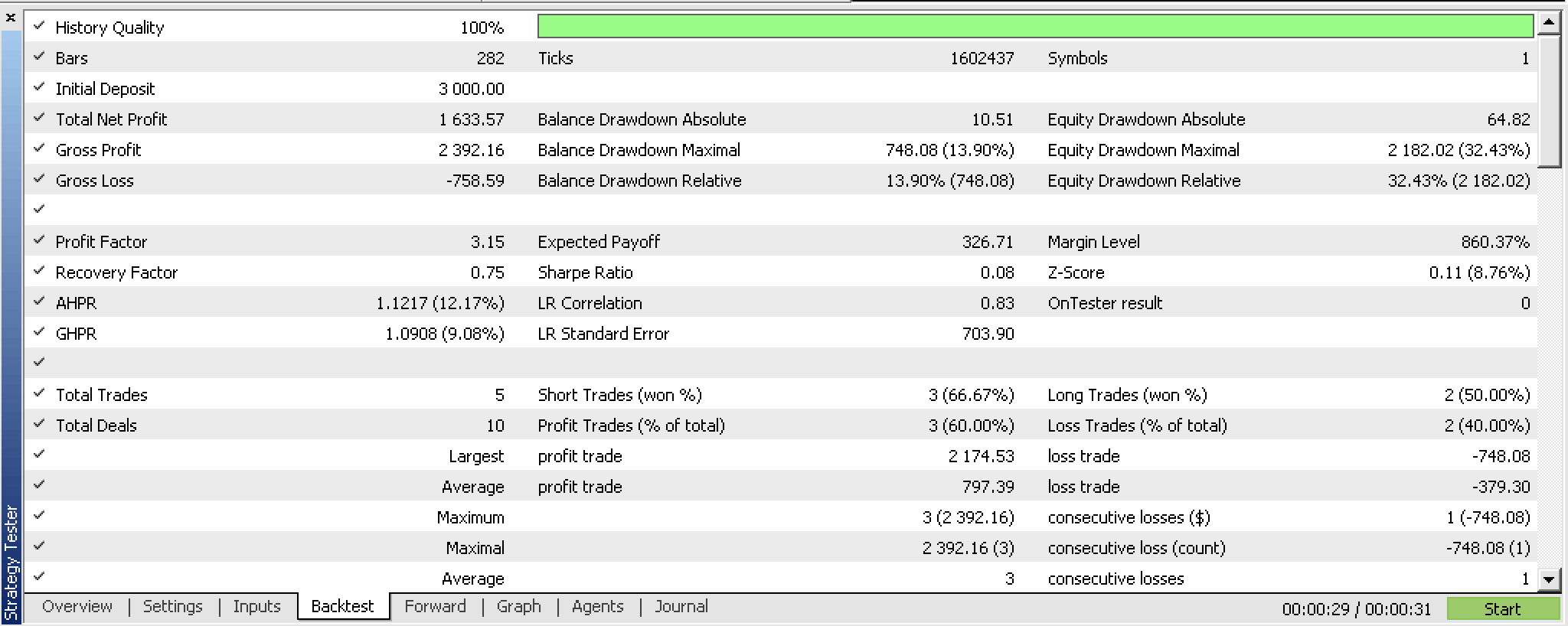
On back testing over the period from 2022.01.01 to 2023.02.01 we do get the following report:

This report relied on these inputs that were got from an optimization run:

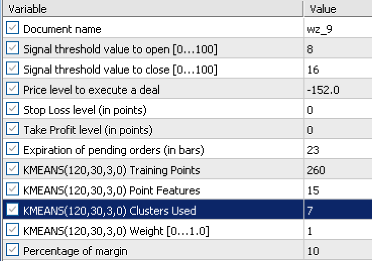
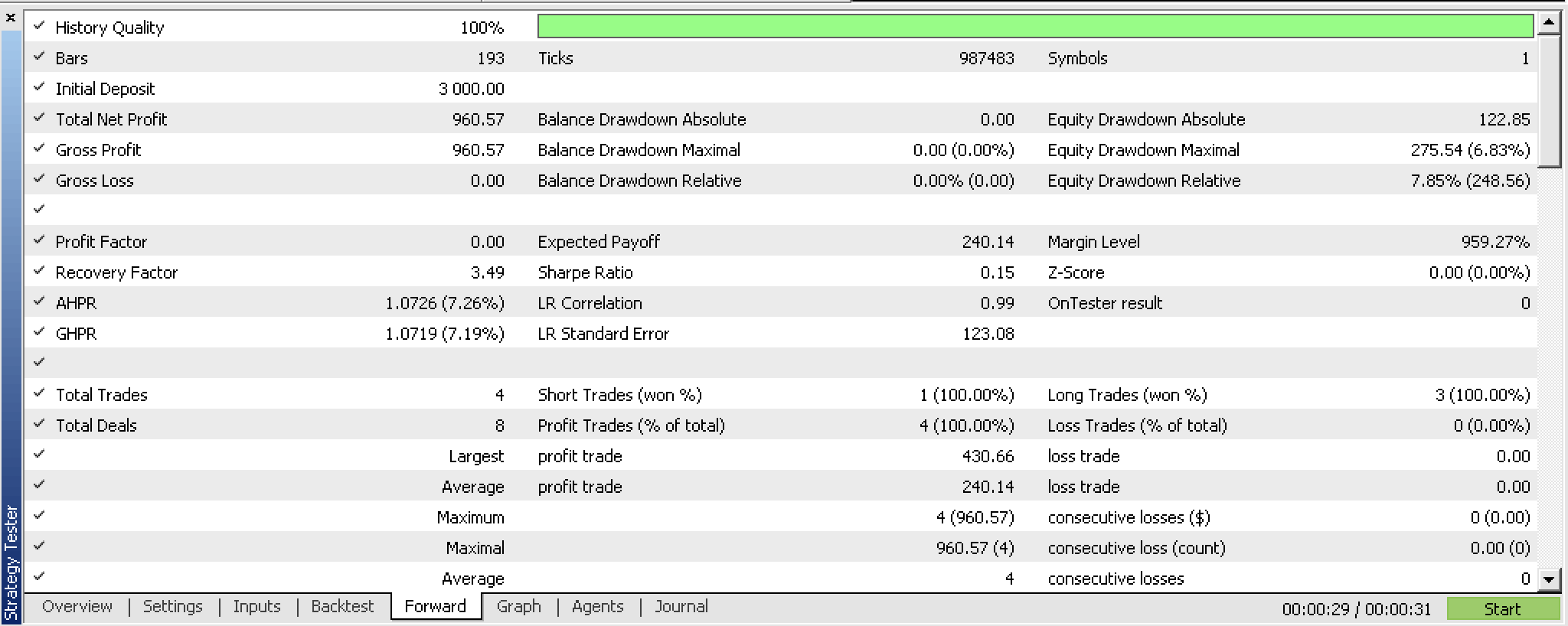
On walking forward with these settings from 2023.02.02 to 2023.10.01 we obtain the following report:

It is a bit promising over this very short test window but as always more diligence and testing over longer periods is recommended.

Implementing with Fractal Waves

Let’s consider now an option that uses data from the fractals indicator as opposed to changes in close price. The fractals indicator is a bit challenging to use out of box especially when trying to implement it with an expert advisor because the buffers when refreshed do not contain indicator values or prices, at each index. You need to check each buffer index and see if there is indeed a ‘fractal’ (i.e. price) and if it does not have a ‘fractal’, the default place holder is the maximum double value. This is how we are preparing the fractal data within the revised ‘GetOutput’ function:

//+------------------------------------------------------------------+
//| Get k-means cluster output from identified cluster.              |
//+------------------------------------------------------------------+
double CSignalKMEANS::GetOutput()
   {
      ...
      
      int _size=m_training_points+m_point_features+1,_index=0;
      
      for(int i=0;i<m_fractals.Available();i++)
      {
         double _0=m_fractals.GetData(0,i);
         double _1=m_fractals.GetData(1,i);
         
         if(_0!=DBL_MAX||_1!=DBL_MAX)
         { 
            double _v=0.0;
            if(_0!=DBL_MAX){_v=_0;}
            if(_1!=DBL_MAX){_v=_1;}
            if(!m_loaded){ m_wave[_index]=_v; _index++; } 
            else
            {
               for(int i=_size-1;i>0;i--){ m_wave[i]=m_wave[i-1]; }
               m_wave[0]=_v; break;
            }
         }
         
         if(_index>=int(m_wave.Size())){ break; }
      }
      
      if(!m_loaded){ m_loaded=true; }
      
      if(m_wave[_size-1]==0.0){ return(0.0); }

      ...
      
      ...
   }

To get actual price fractals we need to first of all properly refresh the fractal indicator object. Once this is done we need to get the overall number of buffer indices available and this value presents how many indices we need to loop through in a for loop while looking for the fractal price points. In doing so we need to be mindful that the fractal indicator has 2 buffers, indexed 0 and 1. The 0-buffer index is for the high fractals while the 1-index buffer is for the low fractals. This implies within our for loop we’ll have 2 values simultaneously checking these index buffers for fractal price points and when any one of them logs a price (only one of them can register a price at a time) we add this value to our vector ‘m_wave’.

Now typically the number of available fractal indices, which serves as our search limit for fractal price points is limited. Meaning that even though we want to say have a wave buffer of 12 indices, we could end up retrieving only 3 at the first run or on the very first price bar. This then implies that our wave buffer needs to act like a proper buffer that saves whatever price indices it is able to retrieve and waits for when aa new fractal price will be available so it can be added to the buffer. This process will continue until the buffer is filled. And in the mean time because the buffer is not yet filed or initialized, the expert advisor will not be able to process any signals and in essence will be in an initialization phase.

This therefore places importance on the size of buffer to be used in fetching the fractals. Since these fractals are input to the k-means clustering algorithm, with our system of using fractal price changes, this implies the size of this buffer is the sum of the number of training points, the number of features and 1. We add the 1 at the end because even though our input data matrix needs only training point plus features the extra row is the current row of points that are not yet regressed, i.e. for which we do not have a ‘y’ value.

So, this unfortunate diligence is necessary but once we get past this we are provided with price information that is sorted in a wave like pattern. And the thesis here is the changes between each wave apex, the fractal price point, can substitute the close price changes we used in our first implementation.

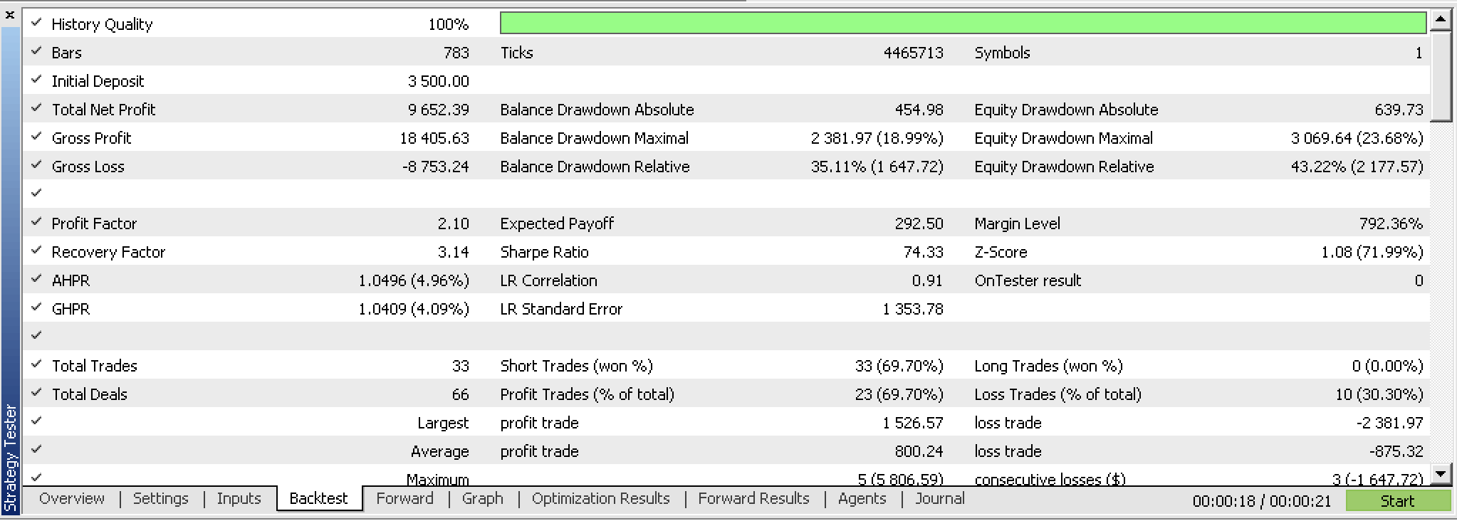
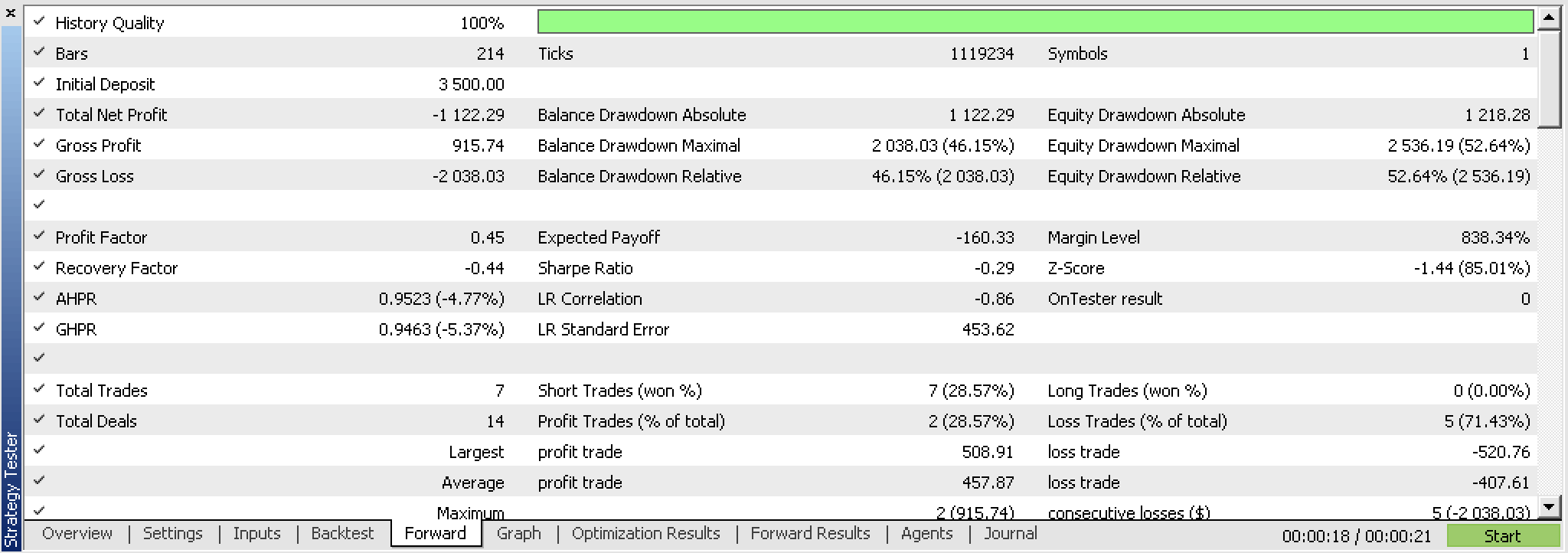
Ironically though on testing this new expert advisor we could not take liberty at not using position price exits (TP & SL) as we did with close price changes and instead had to test with TP. And after testing even though the back test was promising we were not able to get a profitable forward test with the best optimization results as we did with close price changes. Here are the reports.

If we look at the continuous, uninterrupted equity graph of these trades we can clearly see the forward walk is not promising despite a promising first run.

This fundamentally implies that this idea needs review and one starting point in this could be with revisiting the fractal indicator and perhaps having a custom version that is for starters more efficient in that it only has fractal price points, and secondly is customizable with some inputs that guide or quantify the minimum price move between each fractal point.

Conclusion

To sum up we have looked at k-means clustering and how an out of box implementation thanks to AlgLib can be realized in two different settings, with raw close prices and with fractal price data.

Cross validation testing of both settings has, at a preliminary stage, yielded different results with the raw close prices system appearing more promising than the fractal price approach. We have shared some reasons why this is and the source code used in this shared below.

References

Wikipedia

ResearchGate

Appendix

To use the attached source reference to this article on MQL5 wizards could be helpful.